Curve Basics

Some examples require external input files. Before you start, please follow the link in the Example Scripts section to download the zip file with model and result files.

Example 01 - Curves from Expression

This example creates two curves purely based on math expressions. The first curve consists of a sine amplitude. The x-vector of the second curve references to the x vector of the first curve, the y vector oscillates around the fundamental frequency of the first curve.

import hw
import hw.hg as hg
import os

ses = hw.Session()
ses.new()
win = ses.get(hw.Window)
win.type = "xy"

exprXlist = ["0:1:0.0001", "c1.x"]
exprYlist = ["sin(x*2*PI)", "c1.y+0.2*sin(60*x*2*PI)"]
labelList = ["Basic Oscillation 1 HZ", "Overtone 60 HZ"]

for exprX, exprY, label in zip(exprXlist, exprYlist, labelList):
    cu = hg.CurveXY(
        xSource="math",
        xExpression=exprX,
        ySource="math",
        yExpression=exprY,
        label=label,
    )

win.update()

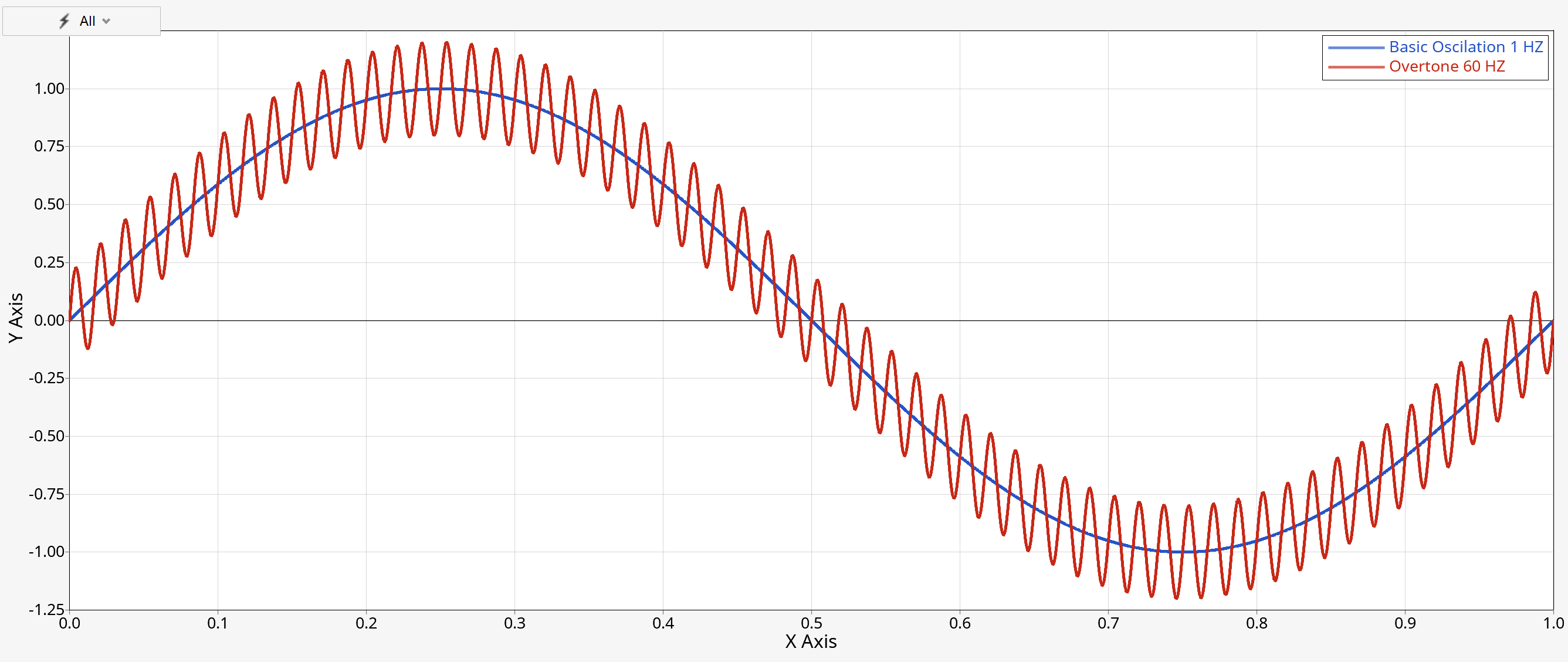
Figure 1. Output of ‘Create two curves from math expressions’

Example 02 - Curves from File

This demo code creates two curves read from a Madymo ANGACC file. The x-vectors of both curves are linked to the Time channel. The y-vectors refer to the channels of the lower and upper torso resultant acceleration. The curve labels consist of Templex expressions which dynamically create the labels based on the selected channel information.

import hw
import hw.hg as hg
import os

ALTAIR_HOME = os.path.abspath(os.environ["ALTAIR_HOME"])
plotFile = os.path.join(
    ALTAIR_HOME, "demos", "mv_hv_hg", "plotting", "madymo", "ANGACC"
)

ses = hw.Session()
ses.new()
win = ses.get(hw.Window)
win.type = "xy"

requestList = ["50th% Hybrid3   - LOWER TORSO", "50th% Hybrid3   - UPPER TORSO"]
colorList = [(255, 0, 0), (0, 0, 255)]

for color, request in zip(colorList, requestList):
    cu = hg.CurveXY(
        xFile=plotFile,
        xSource="file",
        xDataType="Time",
        xRequest="Time",
        xComponent="Time",
        yFile=plotFile,
        ySource="file",
        yDataType="Angular Acceleration",
        yRequest=request,
        yComponent="Res. ang. acc.",
        lineColor=color,
        label="{y.HWRequest} - {y.HWComponent}",
    )

win.update()

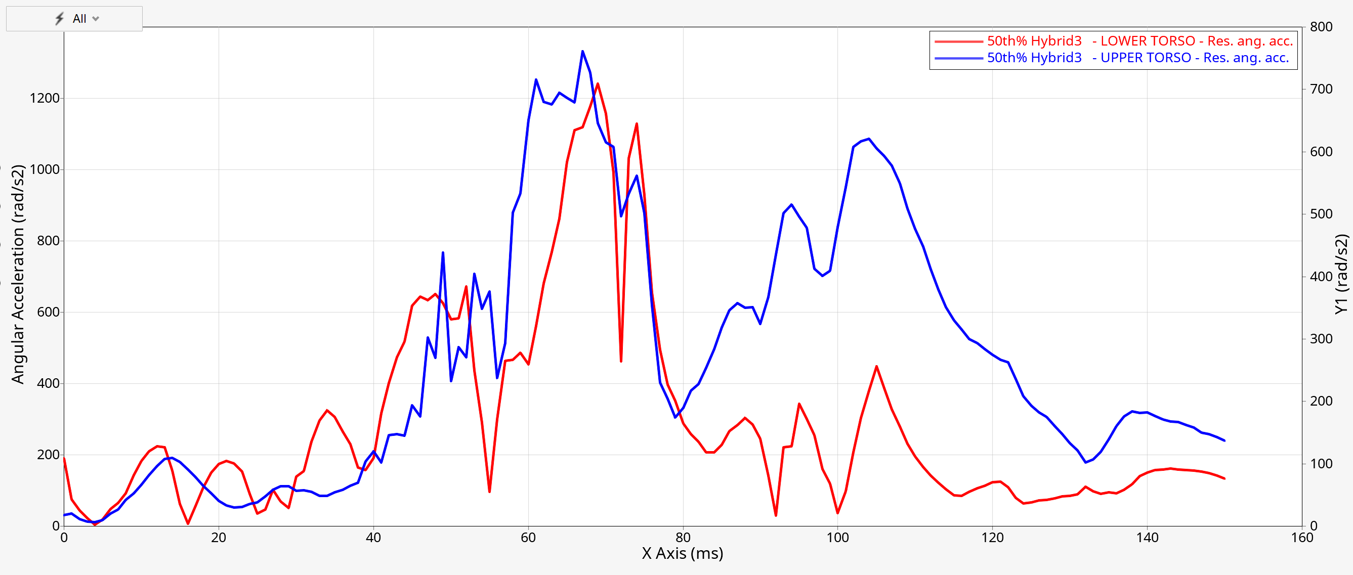
Figure 2. Output of ‘Load two curves from file, define color and label’

Example 03 - Complex Curve

Based on real- and imaginary channels, this code creates the x, y and z translational displacement curves read from a from a sol11 pch-file. The x-vectors of all three curves are linked to the frequency channel, all y-vector channels refer to the same node id. The curve labels consist of Templex expressions which dynamically create the labels based on the selected channel information, the area between the second and third curve is shaded.

import hw
import hw.hg as hg
import os

scriptDir = os.path.abspath(os.path.dirname(__file__))
plotFile = os.path.join(scriptDir, "plot", "control_arm_sol111.pch")

s = hw.Session()
s.new()
# evalHWC('hwd window type="HyperGraph 2D"')
w = s.get(hw.Window)
w.type = "complex"
w.axisMode = "ri"

yrCompList = ["REL | X-Trans", "REL | Y-Trans", "REL | Z-Trans"]
yiCompList = ["IMG | X-Trans", "IMG | Y-Trans", "IMG | Z-Trans"]
colorList = ["#ff0000", "#00ff00", "#0000ff"]

for yrComp, yiComp, color in zip(yrCompList, yiCompList, colorList):
    cu = hg.CurveComplex(
        xFile=plotFile,
        label="{y.HWRequest} - {y.HWComponent}",
        xSource="file",
        xDataType="Frequency [Hz]",
        xRequest="Frequency [Hz",
        xComponent="Frequency [Hz",
        yrFile=plotFile,
        yrSource="file",
        yrDataType="Displacements",
        yrRequest="Point id 2086",
        yrComponent=yrComp,
        yiFile=plotFile,
        yiSource="file",
        yiDataType="Displacements",
        yiRequest="Point id 2086",
        yiComponent=yiComp,
        lineColor=color,
        window=1,
        page=1,
    )

cu.shadeArea = True
cu.shadeStyle = "betweenCurves"
cu.shadeSecondCurve = 2
cu.shadeColor = (0, 0, 0)
cu.shadeAlpha = 0.2

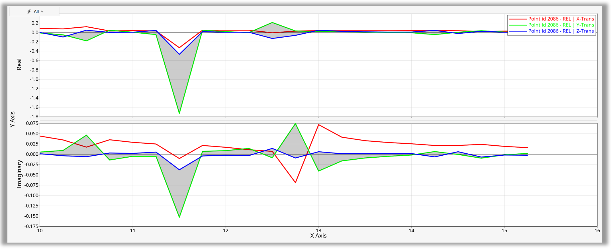
Figure 3. Creating complex curve from file

Example 04 - Bar Charts

The code creates a bar chart with two curves using the CurveBar class constructor. The category x-vector is defined using the Window object of type bar with the Python range function. The first values of this x-vector are replaced using the barSetCategoryValue() method by a list of given strings. The y-vector values refer to the channels of the lower and upper torso resultant accelerations read from a Madymo ANGACC file. As additional formatting the curve color and curve label prefix are customized using the related CurveBar attributes.

import hw
import hw.hg as hg
import os

ALTAIR_HOME = os.path.abspath(os.environ['ALTAIR_HOME'])
plotFile    = os.path.join(ALTAIR_HOME,'demos','mv_hv_hg','plotting','madymo','ANGACC')

ses = hw.Session()
ses.new()
win = ses.get(hw.Window)

win.type = 'bar'

win.barCategoryValues = ([*range(1,20)])
win.barSetCategoryValue(1,['A','B','C','D','E','F','G'])

win.barGap = 10
win.barStyle = 'stack'
win.barCategoryLabelAngle = 'diagonal'
win.barLabelVisibility = True
win.barLabelFormat = 'fixed'
win.barLabelPrecision = 0

# Layout and channel settings
colorList   = [(255,0,0),(0,0,255)]
requestList = ['50th% Hybrid3   - LOWER TORSO','50th% Hybrid3   - UPPER TORSO']
prefixList  = ['A','B']

# Loop over curves, notes and datums
for color,request,pf in zip(colorList,requestList,prefixList):

    bar = hg.CurveBar(yFile=plotFile,
            ySource='file',
            yDataType='Angular Acceleration',
            yRequest=request,
            yComponent='Res. ang. acc.',
            lineColor=color,
            label=request,
            showPrefix=True,
            prefix=pf,
            yOffset=20)

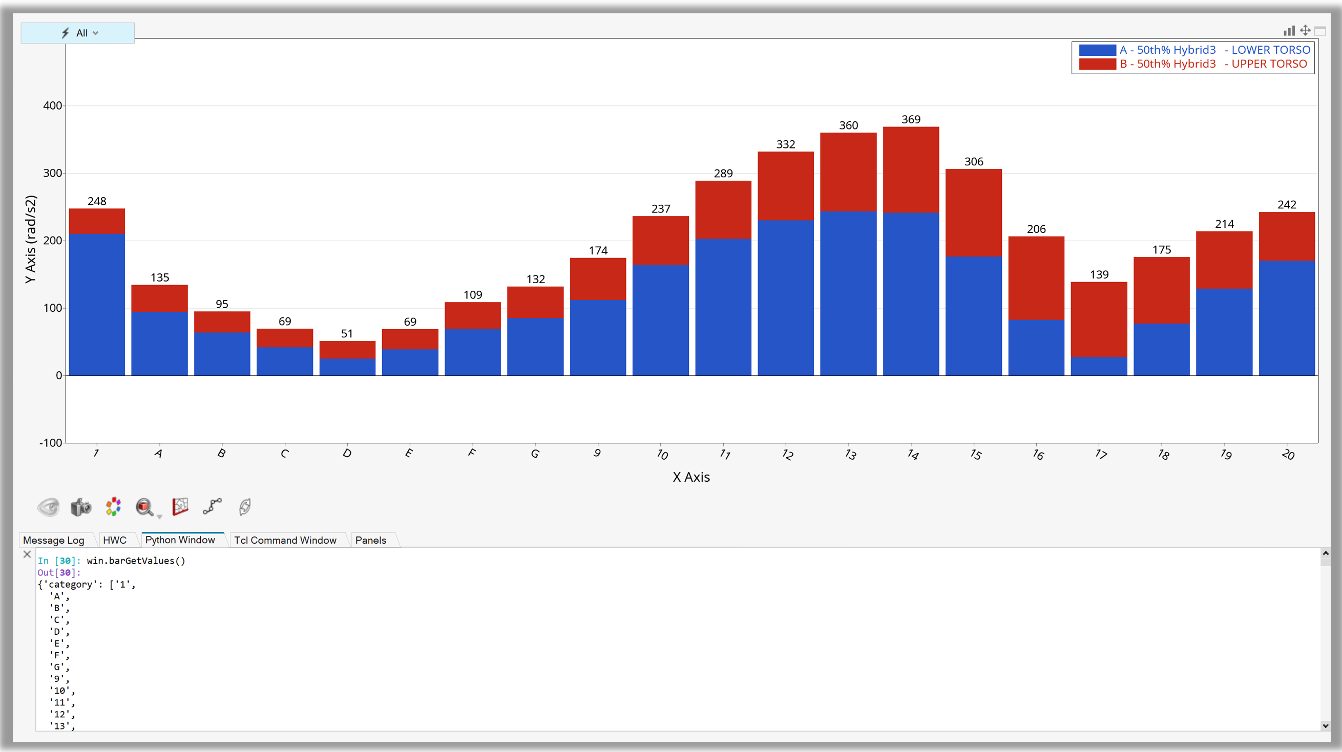
Figure 4. Creating bar charts from file