
Thermal-Electric Battery Simulation Setup and Guidelines
The battery solution is set up with a hierarchical connectivity structure of packs, modules and cells. The core unit is the battery cell, which will be characterized by its specific properties, for example, cathode chemistry and shape. These cell units are connected in series and parallel to form a module, that is, a group of cells, with a desired power output. Finally, the modules are assembled into a pack, with modules connected in series and parallel. These packs are where the overall electrical input/output is provided to the solution.
Battery Packs
- How the modules in a pack are arranged in serial and parallel.
- The type of electrical input to the pack, for example, current, voltage, power or charging profile.

Different types of electrical input can be included as an input to the battery pack using the electrical_input_type command. Although all inputs are done at a pack level these are then distributed to the cell level to ensure consistency of the electrical solution. These are summarized in the following sections.
In general, when the electrical input is provided at the pack level this is required to be distributed to the cell level based on electrical connectivity as well as individual cell properties.
Overview of cell current calculation
If the pack current output is provided as an input, this is required to be distributed to the cell level, since the cells are the source of the voltage that drives the current. To facilitate this distribution in a pack, consistency between the charge conservation solution and ECM models must be maintained. For a 2nd order ECM model, the solution update for the polarization resistor current is given by,
Where is the current flux on the negative terminal of the battery (from the charge conservation PDE solution), and are the polarization resistance of the 1st and 2nd order RC pairs respectively, and are the polarization capacitance of the 1st and 2nd order RC pairs respectively, , , , are diffusion resistor current at time step k and k+1, and is the time step size.
Where , and are the current, fixed voltage (for example, for second order: ) and ohmic resistance in cell , respectively. To determine the current, the voltage, , across a bank of parallel connected cells (PCU), can be determined based on the charging/discharging current ( ) and the cell electrical properties, for example,
The updated cell current, , is then used as a boundary flux in the solution of the charge conservation equation for electrically conducting components connected to the negative terminal of the battery.
The battery solution supports both generic charging and discharging, including constant; piecewise linear; and cubic spline. Constant current discharge would be used for typical testing scenarios. Piecewise linear and cubic spline are used for experimental data such as a driving cycle, for example, NEDC or US06.
- maximum_cell_voltage
- minimum_cell_voltage
- minimum_cell_state_of_charge
- maximum_cell_state_of_charge
These are typically known from a battery specification sheet.
AcuSolve input
BATTERY_PACK( "4S2P battery module" ) {
    number_of_parallel_modules = 2
    number_of_serial_modules = 4
    electrical_input_type = current
    current_type = piecewise_linear
    current_curve_fit_values = Read( "time_current.txt" )
    current_curve_fit_variable = time
}0 0.66809696
9.61104062 0.66809696
12.5842409 0.66809696
13.34691228 15.37136268
…
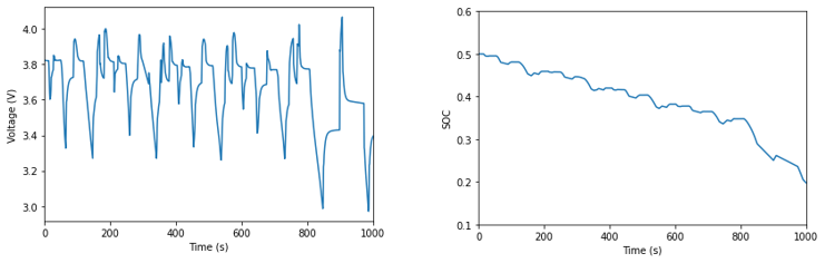
Supports both generic charging and discharging, these include: constant; piecewise_linear; cubic_spline; and c-rate profiles. As with current, constant c-rate discharge would be used for typical testing scenarios. Piecewise linear and cubic spline are used for experimental data such as a driving cycle.
- A battery with a capacity of 3.5Ah discharged at a c rate of 0.5C delivers 1.75A for 2 hours.
- A battery with a capacity of 3.5Ah discharged at a c rate of 1C delivers 3.5A for 1 hour.
- A battery with a capacity of 3.5Ah discharged at a c rate of 2C delivers 7A for 30 mins.
AcuSolve input
BATTERY_PACK( "4s2p battery module" ) {
number_of_parallel_modules = 2
number_of_serial_moudles = 4
electrical_input_type = c_rate
c_rate = 1
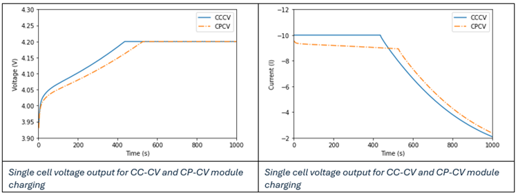
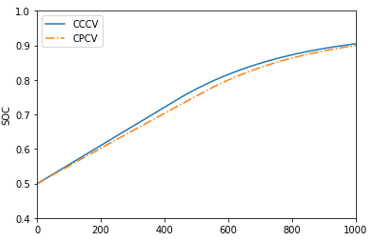
}Charging profiles include CC-CV (Constant Current-Constant Voltage) or CP-CV (Constant Power-Constant Voltage) methods.
In CC-CV charging, the process begins with a constant current (or c-rate) until reaching a specified voltage limit, and then switches to constant voltage charging. The simulation terminates when the current drops to a pre-defined level, for example, cut off current or maximum state of charge. In AcuSolve this is given as a fraction of the original input current. The switch between constant current and constant voltage is defined by the maximum voltage provided on the battery specification data sheet. This is set in the BATTERY_MODULE command (see Battery Module).
In CP-CV charging begins by applying a constant power, shifting to constant voltage once the voltage limit is reached. The termination criteria for CP-CV charging are the same as those for CC-CV.
Sign convention
For charging profiles the current is always negative, since the sign convention in AcuSolve discharge current is positive.
SimLab input
AcuSolve input format
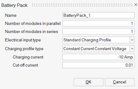
- electrical_input_type = standard_charging_profile
- standard_charging_profile_type = constant_current_constant_voltage
- current/c_rate
- cut_off_current_percent
BATTERY_PACK( "CCCV_pack" ) {
    number_of_parallel_modules = 1
    number_of_serial_modules = 4
    electrical_input_type = standard_charging_profile
    standard_charging_profile_type = constant_current_constant_voltage
    current_type = constant
    current = -20
    cut_off_current_percent = 0.01
}
- electrical_input_type = standard_charging_profile
- standard_charging_profile_type = constant_power_constant_voltage
- power
- cut_off_current_percent
BATTERY_PACK( "CPCV_pack" ) {
    number_of_parallel_modules = 2
    number_of_serial_modules = 4
    electrical_input_type = standard_charging_profile
    standard_charging_profile_type = constant_power_constant_voltage
    power_type = constant
    power = 300
    cut_off_current_percent = 0.01
}
Power input can be provided as a constant power or a profile (piecewise linear and cubic spline). In this approach the power in the pack is calculated.
where is the pack voltage (determined from the cell and module connectivity) and is the pack current at time t. Using the above equation, it is possible to determine the cell current using an iterative approach based on the input power and known open circuit and polarization voltages.
AcuSolve input format
- electrical_input_type = power
- power_type = constant/piecewise_linear/cubic_spline
- power
- cut_off_current_percent
BATTERY_PACK( "Power_pack" ) {
    number_of_parallel_modules = 7
    number_of_serial_moudles = 12
    electrical_input_type = power
    power_type = constant
    power = 1500
}
Constant voltage (CV) is charging with constant voltage. The input module voltage divided by the number of parallel cells should be between the minimum and maximum cell voltage.
AcuSolve input format
- electrical_input_type = voltage
- voltage_type = constant
- voltage
BATTERY_PACK( "Power_pack" ) {
    number_of_parallel_modules = 7
    number_of_serial_modules = 12
    electrical_input_type = voltage
    voltage_type = constant
    voltage = 16
}
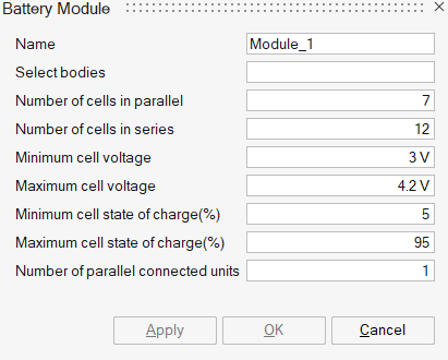
Battery Module
- Number of cells in parallel
- Number of cells connected in parallel in a battery module for each series unit.
- Number of cells in series
- Number of parallel units connected in series.
- Minimum cell voltage
- Minimum allowed voltage of an individual battery cell.
- Maximum cell voltage
- Maximum allowed voltage of an individual battery cell. This avoids overcharging.
- Minimum cell state of charge
- Minimum state of charge at which a battery cell is allowed to operate.
- Maximum cell state of charge
- Maximum state of charge at which a battery cell is allowed to operate.
- Parallel connected units
- The number of parallel connected units (PCU) represents how cells are wired or connected in the module. This parameter only needs to be set when the state of charge differs between cells. More details on this parameter are given below and in the section Cell Electrical Connectivity, Cell Numbering, and Battery Components.
SimLab input
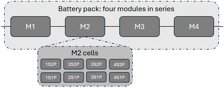
The identification of the electrical bodies, for example, cells, allows for identification of a cell in a pack based on the module number and cell numbering. For example, if the label is M2S1P4, this means that the cell in the pack belongs to module 2 and is the 4th cell in the first parallel bank connected in series. These bodies are added under a separate sub-assembly with a user-given name.
AcuSolve input format
- number_of_parallel_cells = 7
- number_of_serial_cells = 12
- maximum_cell_voltage = 4.2
- minimum_cell_voltage = 3
- maximum_cell_state_of_charge = 0.95
- minimum_cell_state_of_charge = 0.15
- number_of_parallel_connected_units = 1
- battery_pack = "BatteryPack_1"
BATTERY_MODULE( "M1" ) {
    number_of_parallel_cells = 7
    number_of_serial_cells = 12
    maximum_cell_voltage = 4.2
    minimum_cell_voltage = 3
    maximum_cell_state_of_charge = 0.95
    minimum_cell_state_of_charge = 0.15
    number_of_parallel_connected_units = 1
    battery_pack = "BatteryPack_1"
}
The number of BATTERY_MODULE commands depend on the number of modules defined in the BATTERY_PACK command (see Battery Packs).
The number_of_parallel_connected_units can generally be ignored as it has no effect on the solution if the initial state of charge of all the cells in a module is identical. At present, this feature is supported for current and power input. Details of this feature are outlined in Cell Electrical Connectivity, Cell Numbering, and Battery Components.
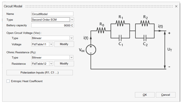
Battery Model
The BATTERY_MODEL specifies the ECM parameters for an individual battery. In the ECM approach, the electric behavior, for example, the voltage-current response, is modeled using a phenomenological electric circuit approach. The parameters for this electric circuit need to be provided, for example, as a function of soc and temperature, in order to model the heat generated from a battery. For example, a 2nd order ECM, that is, two RC pairs, requires the input of the following parameters: capacity, , , and optionally entropic heat.
- First Order ECM
- ECM with a single ohmic resistance in series with one parallel RC pair to represent the dynamic voltage transients (or diffusion voltages).
- Second Order ECM
- ECM with a single ohmic resistance in series with two parallel RC pairs to represent the dynamic voltage transients (or diffusion voltages).
- Third Order ECM
- ECM with a single ohmic resistance in series with three parallel RC pairs to represent the dynamic voltage transients (or diffusion voltages).
The capacity of a battery cell. The coulomb value will be exported as Ah (Amp-hr).
Open circuit voltage is the voltage established between positive and negative terminals when the current is zero, this is, the circuit is open. The type includes Constant, Linear and Bilinear, whereas Constant is a constant open circuit voltage,for Linear, a table can be created which defines the state of charge (soc) versus voltage plot values. For Bilinear, Voltage is specified as a function of both soc and temperature.
Ohmic resistance in the ECM model represents the internal resistance of battery components. The type includes Constant, Linear and Bilinear, whereas Constant is a constant ohmic resistance, for Linear, a table can be created which defines the state of charge (soc) versus resistance plot values. For Bilinear, resistance is specified as a function of both soc and temperature.
Polarization resistance and capacitance in the ECM model describe the dynamic behavior of the battery, for example, ion transport and charge transfer.
Entropic heat coefficient is the derivative of open circuit potential with respect to temperature. It represents reversible heat generation in the battery cell. The type includes Constant, Linear and Bilinear.
BATTERY_MODEL( "CircuitModel" ) {
    battery_model_type = first_order_ecm
    ohmic_resistance_type = piecewise_linear
    ohmic_resistance_curve_fit_values = Read("SIMLAB.DIR/ro.fit" )
    ohmic_resistance_curve_fit_variable = soc
    open_circuit_voltage_type = piecewise_linear
    open_circuit_voltage_curve_fit_values = Read( "SIMLAB.DIR/ocv.fit" )
    open_circuit_voltage_curve_fit_variable = soc
    polarization_resistance1_type = piecewise_linear
    polarization_resistance1_curve_fit_values = Read( "SIMLAB.DIR/r1.fit" )
    polarization_resistance1_curve_fit_variable = soc
    polarization_capacitance1_type = piecewise_linear
    polarization_capacitance1_curve_fit_values = Read( "SIMLAB.DIR/c1.fit" )
    polarization_capacitance1_curve_fit_variable = soc
    battery_capacity = 2.5
}
SimLab interface
Electrical Output Variables
- State of charge (SOC)
- Cell current ( cell current determined based on input loads)
- Cell voltage ( , terminal voltage determined from the solution of the ECM model)
For electrically conducting components the following output variables are provided:
- Electric potential
- For battery packs the electric potential is determined based on the solution of charge conservation combined with the voltage generated by the cells.
- Current density
- The current density is taken directly from the solution of charge
conservation and is given by
- Joule heat density
- Joule heat density is the thermal energy generated due to the passage of
current (electrical energy).
Electrical Boundary Conditions
SimLab interface
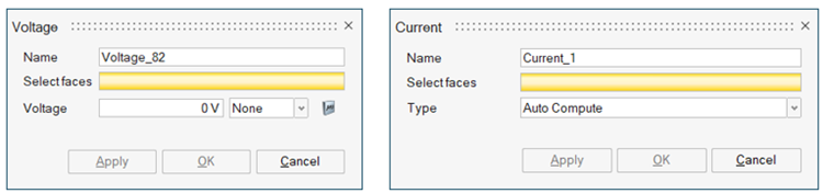
AcuSolve input format
The voltage and current conditions for the charge conservation equation are set under the SIMPLE_BOUNDARY_CONDITION section. The following snippets of the input file show these definitions.
SIMPLE_BOUNDARY_CONDITION(  "Voltage" ) {
    surface_sets = { "Voltage_PartBody.4_1_tet_tria3" }
    type = wall
    ...
    electric_potential_type = value
    electric_potential = 0.0
}SIMPLE_BOUNDARY_CONDITION( "Current" ) {
surface_sets = { "Current_PartBody.3_1_tet_tria3" }
type = wall
...
electric_current_from_module = on
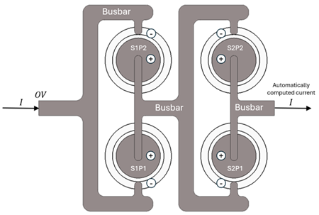
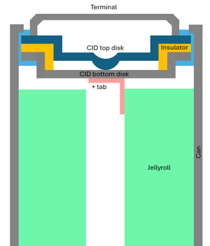
}Cell Electrical Connectivity, Cell Numbering, and Battery Components
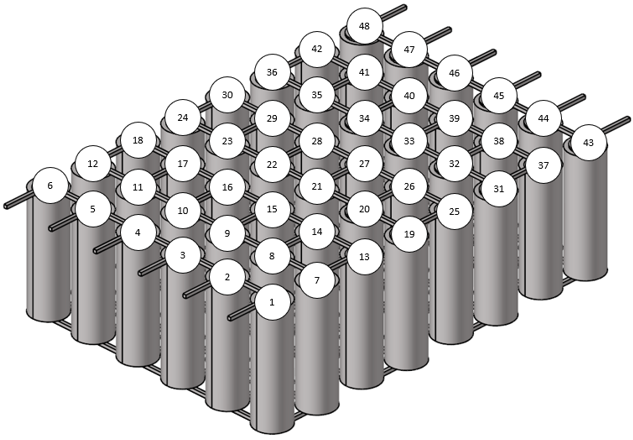
Moreover, each time a new module is created, the cell numbering restarts from one in the AcuSolve input file.
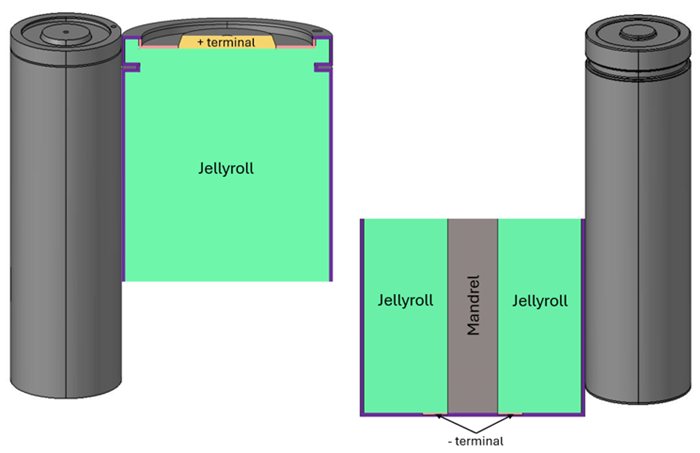
- battery_cell
- Denotes the core of a detailed battery cell, with varying degrees of detail possible, or the battery itself for a homogenized cell with no detailed cell componentry.
- busbar
- The metal connectors linking cells together to carry current.
- tab_positive
- Represents the positive terminal or tab connected to the current collector. It can be depicted by either a solid volume connected to the jellyroll of the cell or a surface between a busbar and the cell.
- tab_negative
- Denotes the negative terminal or tab connected to the current collector. Similar to the positive tab, it can be depicted by either a solid volume connected to the jellyroll of the cell or a surface between a busbar and the cell.
- The +tab set to tab_positive
- CID bottom disk, CID top disk and Terminal would be set to busbar
- Jellyroll is set to battery_cell
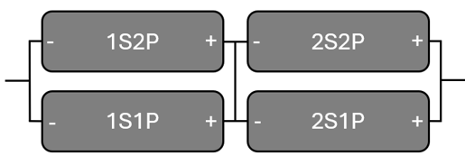
As an example, two 2s2p battery modules connected in series would be labeled as follows:
BATTERY_COMPONENT_MODEL( "M1S1P1" ) {
    component_type = battery_cell
    cell_id = 1
    battery_module = "Module_1"
    isoc = 0.95
}
BATTERY_COMPONENT_MODEL( "M1S1P2" ) {
    component_type = battery_cell
    cell_id = 2
    battery_module = "Module_1"
    isoc = 0.95
}
BATTERY_COMPONENT_MODEL( "M1S2P1" ) {
    component_type = battery_cell
    cell_id = 3
    battery_module = "Module_1"
    isoc = 0.95
}
BATTERY_COMPONENT_MODEL( "M1S2P2" ) {
    component_type = battery_cell
    cell_id = 4
    battery_module = "Module_1"
    isoc = 0.95
}BATTERY_COMPONENT_MODEL( "M2S1P1" ) {
component_type = battery_cell
cell_id = 1
battery_module = "Module_2"
isoc = 0.95
}
BATTERY_COMPONENT_MODEL( "M2S1P2" ) {
component_type = battery_cell
cell_id = 2
battery_module = "Module_2"
isoc = 0.95
}
BATTERY_COMPONENT_MODEL( "M2S2P1" ) {
component_type = battery_cell
cell_id = 3
battery_module = "Module_2"
isoc = 0.95
}
BATTERY_COMPONENT_MODEL( "M2S2P2" ) {
component_type = battery_cell
cell_id = 4
battery_module = "Module_2"
isoc = 0.95
}SimLab interface
The last panel, Cell Naming Order, assigns labels to battery modules within a pack using the standard mSnP convention. Additionally, each module in the pack is identified similarly. For instance, in a battery pack with two modules, the location of the battery in the second parallel and serial position would be M2S2P2.
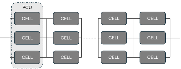
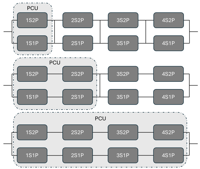
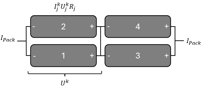
The importance of understanding this connectivity is related to how current distributes through the battery pack when cells (and therefore modules) connected in parallel have cells of differing states. For instance, with a single PCU, it is essential for voltage to be uniform across each cell in the circuit to ensure conservation. This principle also applies to modules connected in parallel. In the AcuSolve battery solution, a rudimentary controller is integrated to balance cell voltages, thereby automatically calculating the current based on the solution derived from charge conservation in the busbars, tabs, and the properties of the cells.