Home
Squeak and Rattle
Create and evaluate evaluation lines and optimize interfaces to eliminate squeak and rattle issues.
Technical Concepts
Technology and problem evaluation approaches used in SnRD.
Rattle Evaluation
Rattle evaluation is based on the assessment of relative displacement between two parts along the defined E-Line. The relative displacement is compared to the gap and tolerance values defined during the pre-processing workflow.
Advanced Rattle
Use the Squeak and Rattle Director Advanced Rattle module to perform different studies regarding the dimensions variation.

Welcome
What's New
View new features for HyperMesh NVH 2025.1.
Get Started
Learn the basics and discover the workspace.
Tutorials
Discover NVH functionality with interactive tutorials.
Full Vehicle NVH
Access the Assemble, Analyze, NVH Tools, NVH Post, and Physics AI ribbons.
High Frequency NVH
High frequency NVH is an implementation of Statistical Energy Analysis (SEA), and is used to predict and analyze the vibration and acoustic response of complex dynamic systems.
Squeak and Rattle
Create and evaluate evaluation lines and optimize interfaces to eliminate squeak and rattle issues.
- Technical Concepts
  Technology and problem evaluation approaches used in SnRD.
  - Rattle Evaluation
    Rattle evaluation is based on the assessment of relative displacement between two parts along the defined E-Line. The relative displacement is compared to the gap and tolerance values defined during the pre-processing workflow.
    - Advanced Rattle
      Use the Squeak and Rattle Director Advanced Rattle module to perform different studies regarding the dimensions variation.
  - Squeak Evaluation
    Squeak evaluation is based on the contact plane relative displacement as per the E-Line method definition, in X and Y local Direction.
  - Root Cause Analysis
    SnRD Post-Processing proposes two modules: Modal Contribution and Modal Sensitivity.
  - Combined Loading
    SnRD solution analyzes squeak and rattles for static and dynamic load types. In the post-processing module, a combined loading module is available to study combination scenarios.
  - Optimization
    Once risk and issue areas are identified and their root cause (mode shapes and frequency), you can setup an optimization solver deck to get solution proposals. Problems are categorized as systematic issues and non-systematic issues.
  - Variabilities Analysis
    SnRD Post Stochastics and DOE module can be used to investigate hundreds of simulation results in a powerful way.
- Launch Squeak and Rattle Director
- Model Build
  Convert rigid connections from a NVH model into flexible connections for squeak and rattle assessment.
- Pre-Processing
  Explore the SnRD Pre-Processing user interface.
- Post Processing
  Launch and explore Squeak and Rattle Director post processing.
- Ziegler PEM Material Database
  Use of Altair Ziegler SnRD Material Database.

View All Altair HyperWorks Help

Advanced Rattle

Use the Squeak and Rattle Director Advanced Rattle module to perform different studies regarding the dimensions variation.

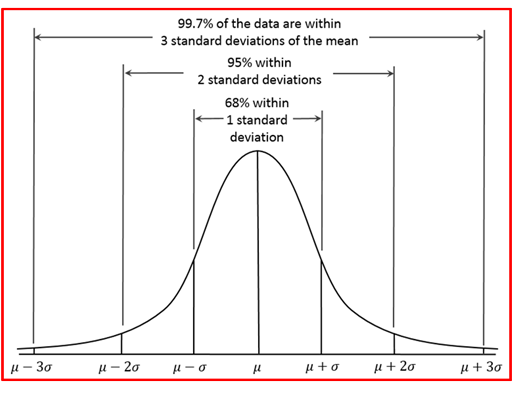
The dimensions variation follows a normal distribution where the nominal gap is the mean value and the tolerance is the standard deviation. By default, three Sigma distribution is applied. A gap will vary from a minimum to a maximum value, which:

Gap min = Nominal Gap ( $µ$ ) – Tolerance ( $3 σ$ )
Gap max = Nominal Gap ( $µ$ ) + Tolerance ( $3 σ$ )

Figure 1.

Sigma Tolerance Plot

The Sigma Tolerance Plot option generates three dynamic tolerance plots, considering tolerance as 1 Sigma, 2 Sigma, and 3 Sigma to highlight the dynamic tolerance risk.

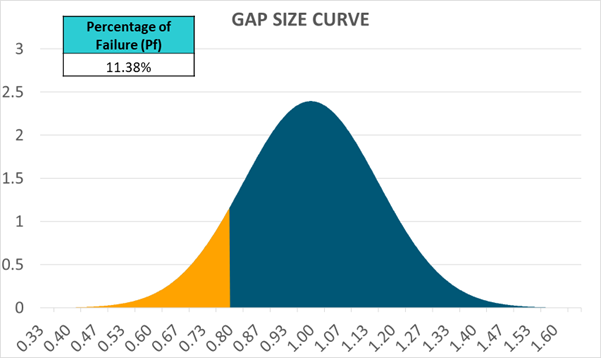
Percentage of Failure

The percentage of failure evaluates the percentage of products to fail in a given production batch. In other words, it represents in how many products in the production the relative displacement exceeds the allowable gap, causing rattle. The relative displacement in gap direction of each E-Line is compared to the gap size distribution curve considering three Sigma distribution. The percentage of failure is calculated as Equation 1.

P_{f} = P r o b a b i l i t y f o r Z_{d i s p} > G a p_{i}

Given the gap, tolerance, and the calculated relative displacement from the FE model, the calculated percentage of failure can be used as an extra filtering index to speed up focusing on the most critical rattle issues. E-Lines with higher percentage of failure have the higher risk of rattling.

The following scenario can be used as an example:

Table 1.
Parameters
Gap	1.00
Tol	0.50
#SD	3.00
$σ$	0.167
Max Rel Disp Z	0.8

Where,

Gap: Nominal gap value
Tol: Tolerance value
#SD: Standard deviation value
Sigma ( $σ$ ): Tol ÷ #SD
Max Rel Disp Z: Maximum relative displacement in Z direction for a specific E-Line extracted from simulation

Using the gap size curve for this calculation, the probability for $G a p_{i} >_{} Z_{d i s p}$ is represented by the blue area in Figure 2 and the percentage of failure by the orange area. Therefore:

P_{f} = P r o b a b i l i t y f o r Z_{d i s p} > G a p_{i}

Figure 2.