Results#
Some examples require external input files. Before you start, please follow the link in the Example Scripts section to download the zip file with model and result files.
Example 01 - Contour Model and Export#
The example code shows how to set the window to HyperView client (type="animation") and display a contour plot of Von Mises composite stress using the ResultDefinitionScalar class. Once the results are plotted, two new objects are created - instances of the ExportModelH3D class and CaptureImageTool class respectively. The exportH3D object is used to export an H3D file containing the displayed results and the captureImage object provides the method to capture a screenshot of the window.
 1import hw
 2import hw.hv as hv
 3import os
 4
 5scriptDir = os.path.abspath(os.path.dirname(__file__))
 6modelFile = os.path.join(scriptDir, "aerobox", "aerobox.fem")
 7resultFile = os.path.join(scriptDir, "aerobox", "aerobox-LC1-2.op2")
 8h3dFile = os.path.join(scriptDir, "demo_model_export.h3d")
 9jpgFile = os.path.join(scriptDir, "demo_image_export.jpeg")
10
11ses = hw.Session()
12ses.new()
13win = ses.get(hw.Window)
14win.type = "animation"
15
16win.addModelAndResult(model=modelFile, result=resultFile)
17res = ses.get(hv.Result)
18resScalar = hv.ResultDefinitionScalar(
19    dataType="Composite Stress",
20    dataComponent="vonMises",
21    layer="Max"
22)
23res.plot(resScalar)
24
25exportH3D = hv.ExportModelH3D(
26    animation=True,
27    previewImage=False,
28    compressOutput=True,
29    compressionLoss=0.05,
30    file=h3dFile,
31)
32
33captureImage = hw.CaptureImageTool(
34    type="jpg",
35     width=3000,
36    height=2000,
37    file=jpgFile
38)
39
40animTool = hw.AnimationTool()
41animTool.currentFrame = 1
42
43hw.evalHWC("view orientation iso")
44exportH3D.export()
45captureImage.capture()
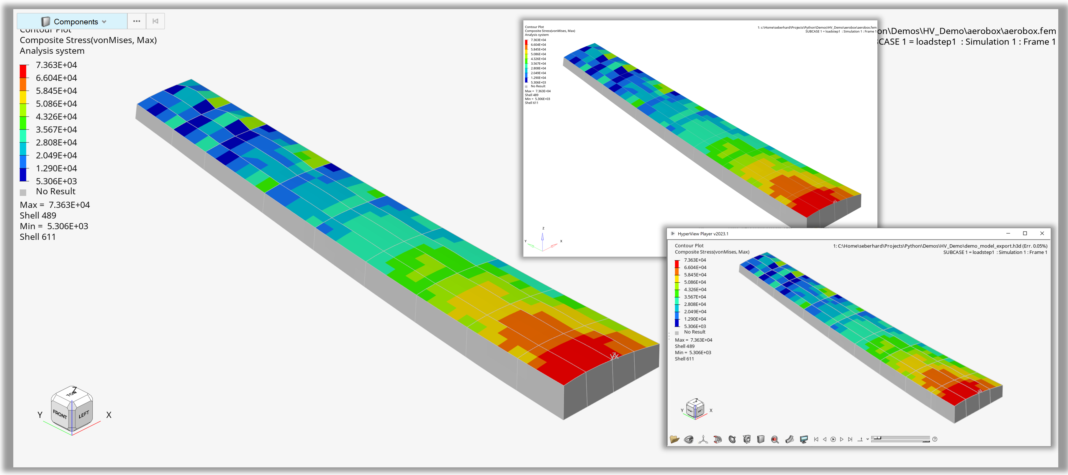
Figure 1. Output of ‘Contour Model and Export’
Example 02 - Macro with GUI#
The Macro with GUI example consists of two main functions - MyCustomGui() and postprocAuto().
MyCustomGui() generates a custom dialog using the Dialog class with the following widgets:
OpenFileEntryto specify the model fileOpenFileEntryto specify the result fileChooseDirEntryto specify the output directoryButtonto provide the close functionButtonto provide the run function
The widgets are organized into a vertical frame using the VFrame class. The example also includes code to automatically populate the file paths for demo purposes.
postprocAuto() provides the postprocessing logic. Two new objects are created at the start: capture for screenshot generation and exportH3D for H3D file export. This is followed by the definition of two dictionaries: resDict contains list of data components for four different data types and legDict contains legend settings for each of the four data types. These dictionaries are used in nested loops to generate a page per data type, each page containing four windows (layout=9), one window per data component.
  1import hw
  2import hw.hv as hv
  3from hwx.xmlui import gui
  4from hwx import gui as gui2
  5import os
  6
  7def MyCustomGui():
  8
  9    # Method called on clicking 'Close'.
 10    def onClose(event):
 11        dialog.Hide()
 12
 13    def onRun(event):
 14        dialog.Hide()
 15        postprocAuto(modelFile.value, resultFile.value, folderSel.value)
 16        gui2.tellUser("Done!")
 17
 18    label1 = gui.Label(text="Model File")
 19    modelFile = gui.OpenFileEntry(placeholdertext="Model File")
 20    label2 = gui.Label(text="Result File")
 21    resultFile = gui.OpenFileEntry(placeholdertext="Result File")
 22    label3 = gui.Label(text="Screenshot Folder")
 23    folderSel = gui.ChooseDirEntry(tooltip="Select output directory")
 24
 25    close = gui.Button("Close", command=onClose)
 26    create = gui.Button("Run", command=onRun)
 27
 28    # Default file settings for quick demo purposes
 29    if True:
 30        src_path = os.path.dirname(os.path.abspath(__file__))
 31        modelFile.value = os.path.join(src_path, "aerobox", "aerobox.fem").replace(
 32            "\\", "/"
 33        )
 34        resultFile.value = os.path.join(
 35            src_path, "aerobox", "aerobox-LC1-2.op2"
 36        ).replace("\\", "/")
 37        folderSel.value = os.path.join(src_path, "outDir").replace("\\", "/")
 38
 39    mainFrame = gui.VFrame(
 40        (label1, 20, modelFile),
 41        (label2, 20, resultFile),
 42        (label3, 20, folderSel),
 43        (create, close),
 44    )
 45
 46    dialog = gui2.Dialog(caption="Post Automation")
 47    dialog.addChildren(mainFrame)
 48    dialog.width = 400
 49    dialog.height = 100
 50    dialog.show()
 51
 52
 53def postprocAuto(modelPath, resultPath, outDir):
 54
 55    # Create Session Pointer
 56    ses = hw.Session()
 57    # New
 58    ses.new()
 59
 60    # Define Capture Image Tool
 61    capture = hw.CaptureImageTool()
 62    capture.type = "jpg"
 63    capture.width = 1200
 64    capture.height = 800
 65
 66    # Define H3D export
 67    exportH3D = hv.ExportModelH3D(
 68        animation=True, previewImage=False, compressOutput=True, compressionLoss=0.05
 69    )
 70
 71    # Dictionary with dataType dependent result scalar settings
 72    resDict = {
 73        "Displacement": ["Mag", "X", "Y", "Z"],
 74        "Composite Stress": ["vonMises", "P1 (major)", "P2 (mid)", "P3 (minor)"],
 75        "Composite Strain": ["vonMises", "XX", "YY", "ZZ"],
 76        "Stress": [
 77            "vonMises",
 78            "MaxShear",
 79            "In-plane P1 (major)",
 80            "In-plane P2 (minor)",
 81        ],
 82    }
 83
 84    # Dictionary with dataType dependent legend settings (precision, numerical format,
 85    legDict = {
 86        "Displacement": [5, "scientific", 2],
 87        "Composite Stress": [6, "engineering", 4],
 88        "Composite Strain": [7, "fixed", 6],
 89        "Stress": [10, "engineering", 2],
 90    }
 91    # Change window type
 92    ses.get(hw.Window).type = "animation"
 93
 94    startPageId = ses.get(hw.Page).id + 1
 95
 96    # Loop over data types, 1 page per data type
 97    for dType in list(resDict.keys()):
 98        ap = hw.Page(title=dType, layout=9)
 99        ses.setActive(hw.Page, page=ap)
100
101        # Loop over data components, one window per component
102        for i, w in enumerate(ses.getWindows()):
103            dComp = resDict.get(dType)[i]
104            ses.setActive(hw.Window, window=w)
105
106            # Load Model
107            w.addModelAndResult(model = modelPath, result=resultPath)
108
109            # Set scalar results
110            res = ses.get(hv.Result)
111            resScalar = ses.get(hv.ResultDefinitionScalar)
112            resScalar.setAttributes(dataType=dType, dataComponent=dComp)
113
114            # Plot results
115            res.plot(resScalar)
116
117            # Define legend settings
118            leg = ses.get(hv.LegendScalar)
119            leg.setAttributes(
120                numberOfLevels=legDict.get(dType)[0],
121                numericFormat=legDict.get(dType)[1],
122                numericPrecision=legDict.get(dType)[2],
123            )
124
125            # Define ISO settings
126            resIso = ses.get(hv.ResultDefinitionIso)
127            resIso.setAttributes(dataType=dType, dataComponent=dComp)
128            dispIso = ses.get(hv.ResultDisplayIso)
129            res.plotIso(resIso)
130
131            # Set ISO value dependent on min/max
132            dispIso.value = leg.minValue + (leg.maxValue - leg.minValue) / 5
133
134            # Set animation frame 1
135            animTool = hw.AnimationTool()
136            animTool.currentFrame = 1
137
138            # Capture jpg
139            jpgPath = os.path.join(outDir, dType + " - " + dComp + "_iso_view.jpg")
140            capture.file = jpgPath
141            capture.capture()
142
143            # Capture H3D
144            h3dPath = os.path.join(outDir, dType + " - " + dComp + ".h3d")
145            exportH3D.setAttributes(file=h3dPath, window=w)
146            exportH3D.export()
147
148            # Use Model, Collection and Part class to isolate component
149            if True:
150                mod = ses.get(hv.Model)
151                col = hv.Collection(hv.Part)
152                mod.hide(col)
153                mod.get(hv.Part, 172).visibility = True
154            # Use evalHWC isolate component for export
155            else:
156                hw.evalHWC("hide component all")
157                hw.evalHWC("show component 172")
158
159            # Set Views and export
160            hw.evalHWC("view orientation left")
161            jpgPath = os.path.join(outDir, dType + " - " + dComp + "_left_view.jpg")
162            capture.file = jpgPath
163            hw.evalHWC("show component all")
164            hw.evalHWC("view orientation iso")
165
166    ses.setActive(hw.Page, id=startPageId)
167
168
169if __name__ == "__main__":
170    MyCustomGui()
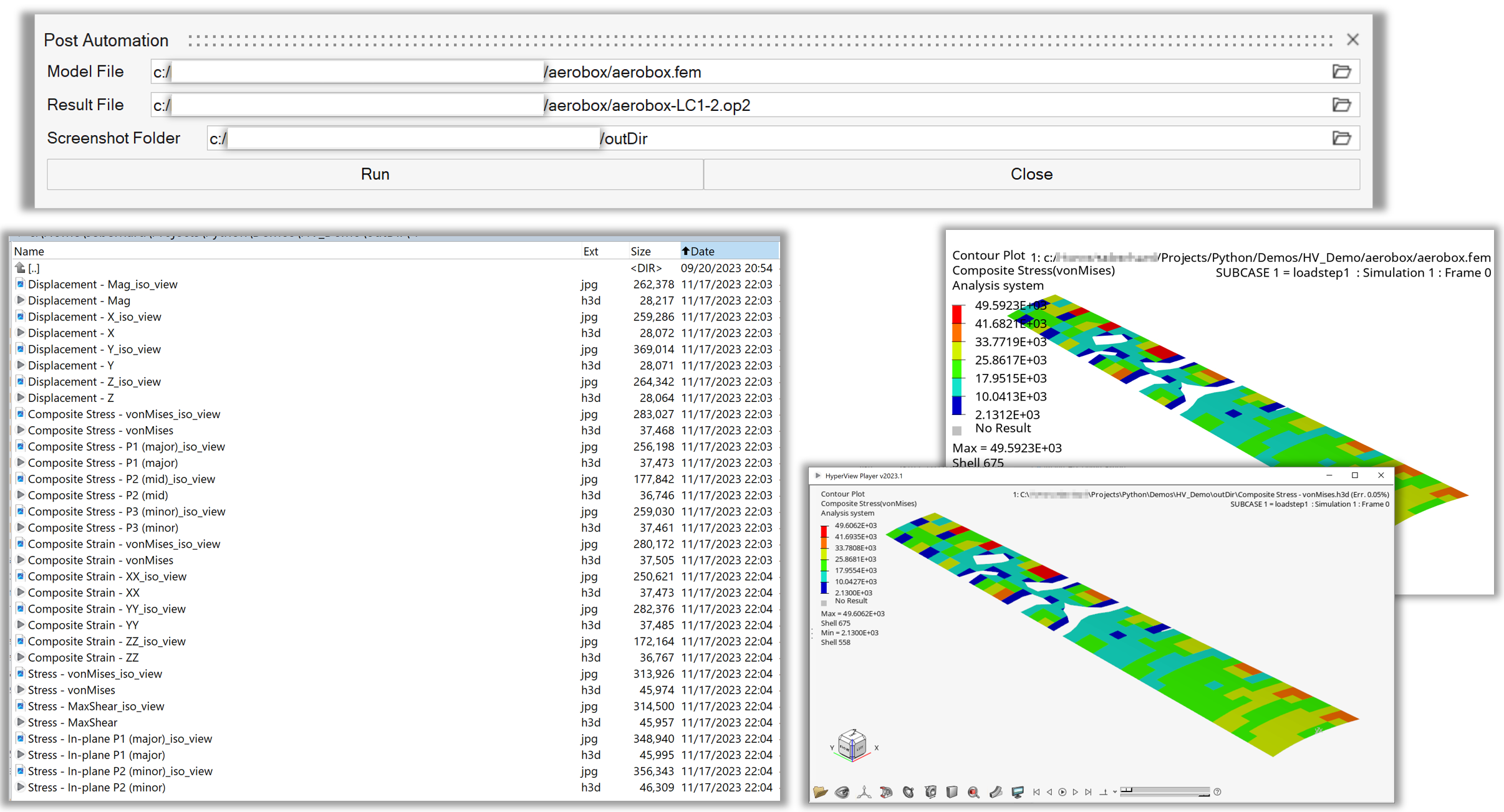
Figure 2. Start GUI and exported images / H3D’s of ‘Macro with GUI’
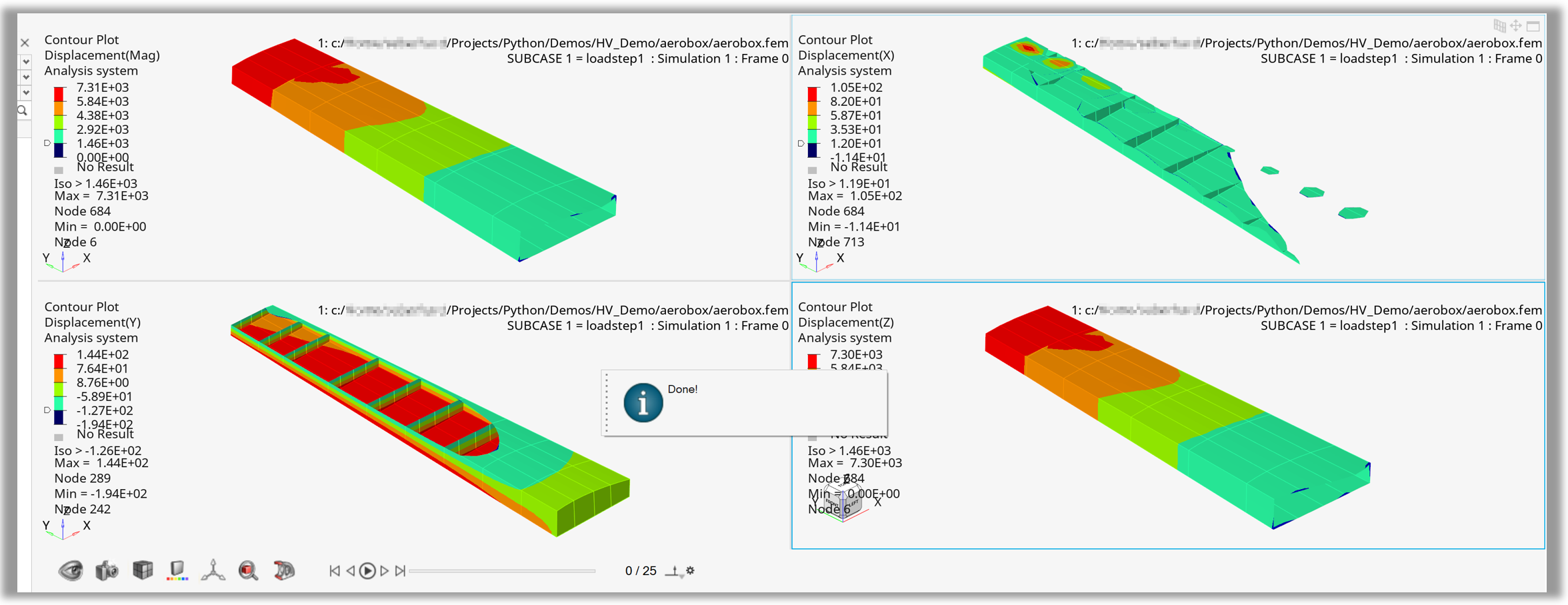
Figure 3. hw.Page created for one data type by ‘Macro with GUI’
Example 03 - Contour Maximum by Sphere#
After the standard steps (setting up the window, loading the model/result files, and contouring the results), the example shows the user how to select elements around the element with the maximum contour plot value using FilterBySphere. It proceeds with setting up custom properties of the legend, including custom header font. It then displays the contour plot only on the entities inside the sphere collection. Finally, it creates a note using the HWC commands, sets the results to the first animation frame and puts the model into an iso orientation.
 1import hw
 2import hw.hv as hv
 3import os
 4
 5scriptDir = os.path.abspath(os.path.dirname(__file__))
 6modelFile = os.path.join(scriptDir, "aerobox", "aerobox.fem")
 7resultFile = os.path.join(scriptDir, "aerobox", "aerobox-LC1-2.op2")
 8
 9hotspotRadius = 400
10
11# Load Model
12ses = hw.Session()
13ses.new()
14page = ses.get(hw.Page)
15win = ses.get(hw.Window)
16win.type = "animation"
17win.addModelAndResult(model=modelFile, result=resultFile)
18
19# Contour scalar
20res = ses.get(hv.Result)
21resScalar = ses.get(hv.ResultDefinitionScalar)
22resScalar.setAttributes(
23    dataType="Composite Stress", dataComponent="vonMises", layer="Max"
24)
25res.plot(resScalar)
26
27# Create Collection via TopN filter
28maxElemCol = hv.Collection(hv.Element, populate=False)
29elemFilter = hv.FilterByScalar(operator="topN", value=1)
30maxElemCol.addByFilter(elemFilter)
31
32# Get centroid of element with maximum scalar value
33maxElem = maxElemCol.getEntities()[0]
34centroid = maxElem.centroid
35
36# Create collection with given radius
37sphereCol = hv.Collection(hv.Element, populate=False)
38sphereFilter = hv.FilterBySphere(
39    x=centroid[0],
40    y=centroid[1],
41    z=centroid[2],
42    radius=hotspotRadius
43)
44sphereCol.addByFilter(sphereFilter)
45
46# Define font
47headFont = hw.Font(size=14, style="bold")
48
49# Modify legend
50legend = ses.get(hv.LegendScalar)
51legend.setAttributes(
52    headerText="Hostpot Radius = " + str(hotspotRadius),
53    headerVisible=True,
54    headerFont=headFont,
55    numberOfLevels=8,
56    numericFormat="fixed",
57    numericPrecision=0,
58)
59
60# Contour only sphere collection
61resScalar.collection = sphereCol
62res.plot(resScalar)
63
64# Attach max note with evalHWC
65maxId = str(maxElem.id)
66maxLabel = "Max Element " + maxId
67hw.evalHWC('annotation note create "' + maxLabel + '"')
68hw.evalHWC('annotation note "'
69        + maxLabel
70        + '" attach entity element '
71        + maxId
72)
73hw.evalHWC(
74    'annotation note "'
75    + maxLabel
76    + '" \
77    display text= "Max Element: {entity.id}\\nMax Value: {entity.contour_val}" \
78    movetoentity=true \
79    filltransparency=false \
80    fillcolor="255 255 255"'
81)
82
83# Set frame with AnimationTool()
84animTool = hw.AnimationTool()
85animTool.currentFrame = 1
86
87# Modify view with evalHWC
88hw.evalHWC("view orientation iso")
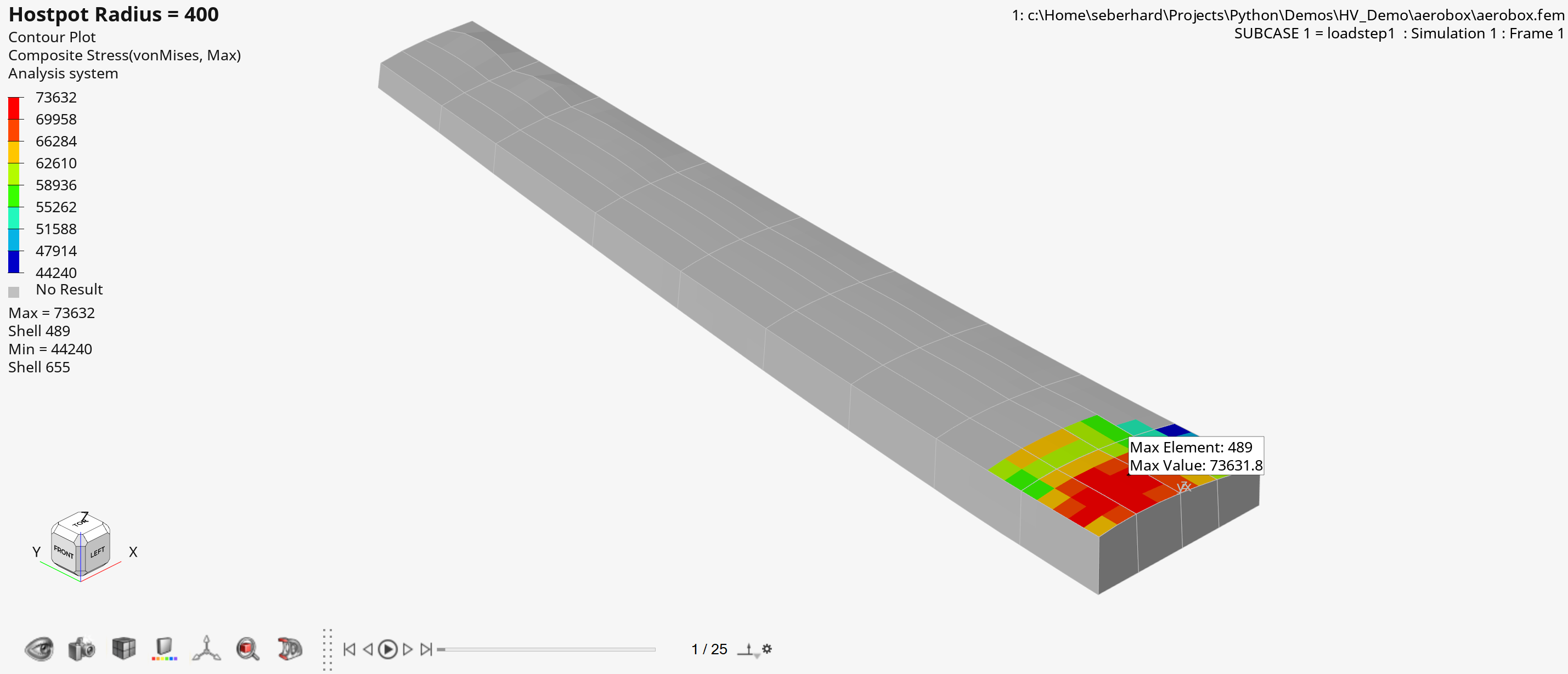
Figure 4. Output of ‘Contour Maximum by Sphere
Example 04 - Query Result Data with Default Settings#
The example shows how to set up a contour, vector, and tensor plot, followed by the querying of the displayed results using QueryResultsTool. An instance of this class is created and the result data is extracted into a Numpy array using the query() method. The default settings/attribute of the QueryResultsTool object are used.
 1import hw
 2import hw.hv as hv
 3import os
 4
 5ALTAIR_HOME = os.path.abspath(os.environ['ALTAIR_HOME'])
 6modelFile   = os.path.join(ALTAIR_HOME,'demos','mv_hv_hg','animation','dyna','bumper','bumper_deck.key')
 7resultFile  = os.path.join(ALTAIR_HOME,'demos','mv_hv_hg','animation','dyna','bumper','d3plot')
 8
 9# Load Model/Results
10ses = hw.Session()
11ses.new()
12win = ses.get(hw.Window)
13win.type = 'animation'
14win.addModelAndResult(model=modelFile, result=resultFile)
15
16# Set scalar, vector and tensor results
17res = ses.get(hv.Result)
18resScalar = hv.ResultDefinitionScalar(dataType='Stress',
19                dataComponent='vonMises')
20res.plot(resScalar)
21resVector = hv.ResultDefinitionVector(dataType='Stress')
22res.plot(resVector)
23resTensor = hv.ResultDefinitionTensor(dataType='Stress')
24resTensor.format = 'component'
25resTensor.setComponentStatus(xx=True,yy=True,zz=True,xy=True,yz=True,zx=True)
26res.plot(resTensor)
27
28# Set View
29hw.evalHWC('view projection orthographic | view matrix -0.021537 0.988942 0.146732 0.000000 0.872753 0.090190 -0.479758 0.000000 -0.487686 0.117728 -0.865045 0.000000 -99.918198 345.190369 584.070618 1.000000 | view clippingregion -284.806213 129.713852 528.670959 864.158752 -722.333801 601.748169')
30
31# Set time step
32animTool = hw.AnimationTool()
33animTool.currentFrame = res.getSimulationIds()[-2]
34win.draw()
35print('')
36print('Query with Defaults')
37print('-------------------')
38
39# Create Query Result Tool
40queryTool = hv.QueryResultsTool()
41print('Data Source Info:')
42
43# Get available data source info array
44dataSourceInfoArray = queryTool.getDataSourceInfo()
45print(dataSourceInfoArray)
46
47# Query NumPy with default settings
48queriedData = queryTool.query()
49print('')
50
51# Get data source query created by default
52dataSource = queryTool.getDataSourceQuery()
53print('Default data source query = {}'.format(dataSource))
54
55# Get default collection
56entCol = queryTool.collection
57print('Size of default {} collection = {}'.format(entCol.entityType,entCol.getSize()))
58print('')
59
60# NumPY array
61print('NumPy Array:')
62print('Length numpy array = {}'.format(len(queriedData)))
63print(queriedData)
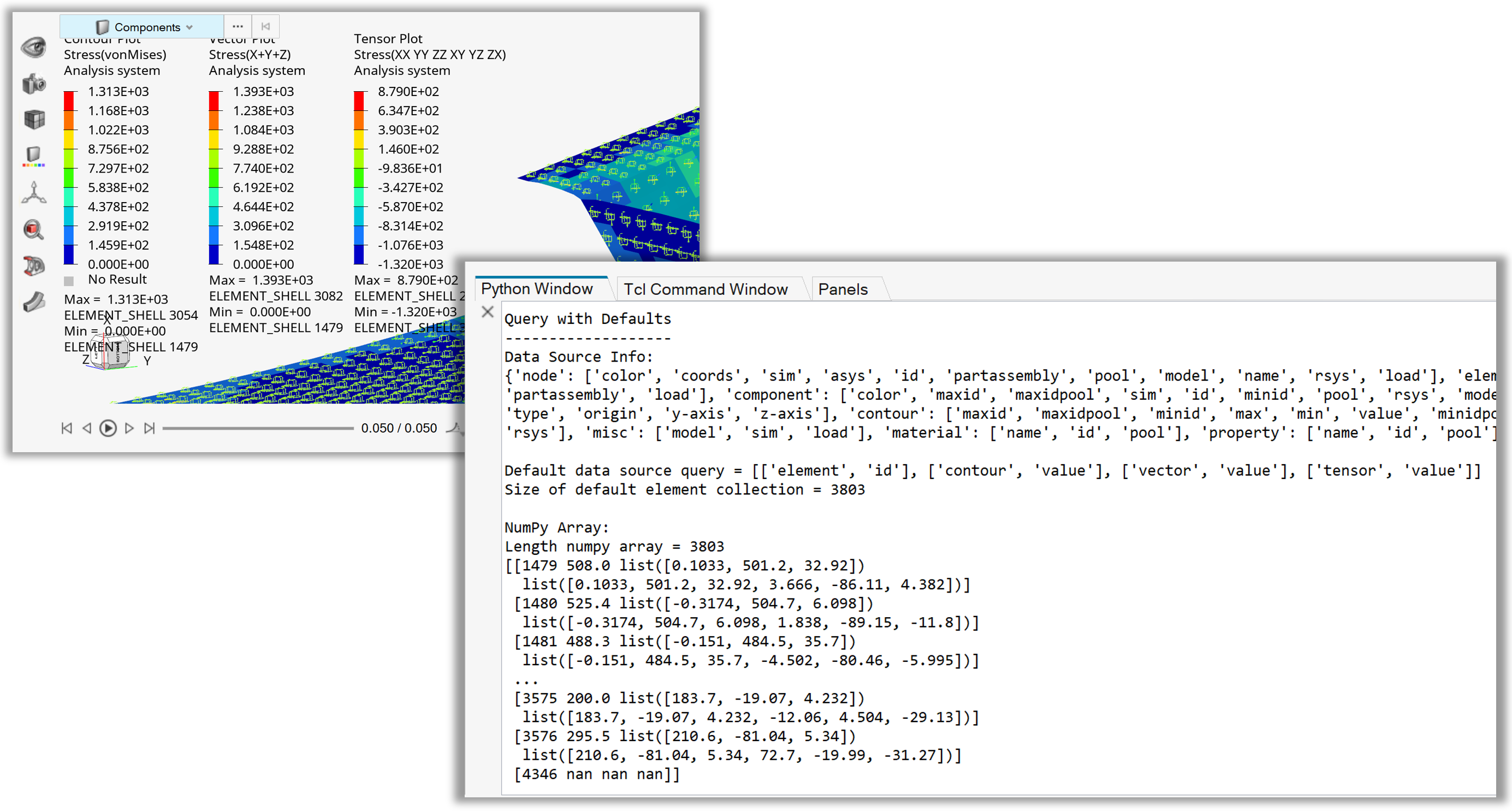
Figure 5. Console output of query NumPy array with default settings
Example 05 - Query Result Data with Custom Query#
After the standard steps (setting up the window, loading the model/result files, and contouring the results), the example shows how to create a collection of elements with the scalar value greater than 100 using FilterByScalar. This collection is used as the input for the QueryResultsTool object in order to extract the data only for a specific entity selection. The queried data is defined via the setDataSourceQuery() method and extracted into a Numpy array using the query() method.
 1import hw
 2import hw.hv as hv
 3import os
 4
 5ALTAIR_HOME = os.path.abspath(os.environ['ALTAIR_HOME'])
 6modelFile   = os.path.join(ALTAIR_HOME,'demos','mv_hv_hg','animation','dyna','bumper','bumper_deck.key')
 7resultFile  = os.path.join(ALTAIR_HOME,'demos','mv_hv_hg','animation','dyna','bumper','d3plot')
 8
 9# Load Model/Results
10ses = hw.Session()
11ses.new()
12win=ses.get(hw.Window)
13win.type = 'animation'
14win.addModelAndResult(model=modelFile, result=resultFile)
15
16# Set scalar results
17res = ses.get(hv.Result)
18resScalar = hv.ResultDefinitionScalar(dataType='Stress',
19                dataComponent='vonMises')
20res.plot(resScalar)
21
22animTool = hw.AnimationTool()
23animTool.currentFrame = 1
24win.draw()
25
26# Create element collection
27elemCol = hv.Collection(hv.Element,populate=False)
28
29# Add all elements with a value > 0
30valFilter = hv.FilterByScalar(operator='>',value=100)
31elemCol.addByFilter(valFilter)
32
33# Create Query Result Tool
34queryTool =  hv.QueryResultsTool()
35
36# Set Element Collection
37queryTool.collection = elemCol
38print('')
39queryTool.setDataSourceQuery(
40    [['element', 'id'],
41    ['contour', 'value'],
42    ['element','config'],
43    ['component','pool'],
44    ['component','name'],
45    ['element','normal']]
46)
47
48# Data source query
49print('Data source query = {}'.format(queryTool.getDataSourceQuery()))
50
51# Query NumPy array
52queriedData = queryTool.query()
53print('')
54
55# Get default collection
56print('Size of {} collection with value > 0 = {}'.format(elemCol.entityType,elemCol.getSize()))
57print('')
58
59# NumPY array
60print('NumPy Array:')
61print('Length numpy array = {}'.format(len(queriedData)))
62print(queriedData)
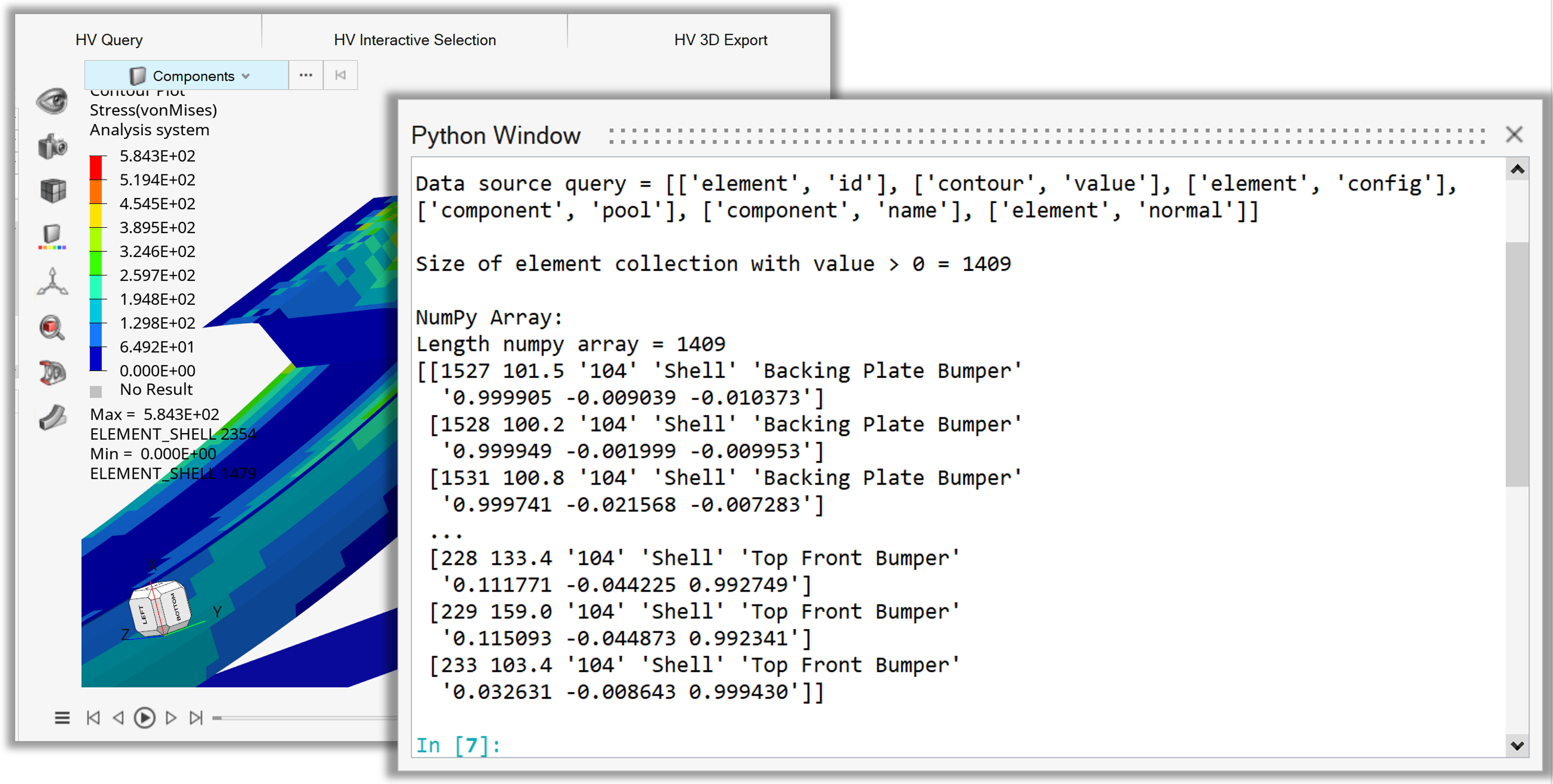
Figure 6. Console output of query NumPy array with custom query