Tutorial Level: Advanced This tutorial uses OptiStruct's topology optimization
functionality to generate a design for a cooling channel of a Battery Pack and show how
Darcy Flow analysis is used for the design.
Before you begin, copy the file(s) used in this tutorial to your
working directory.
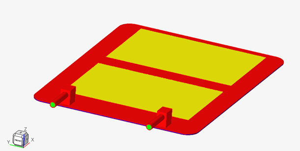
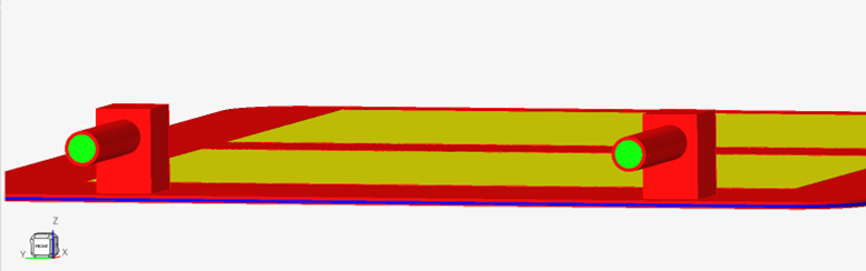
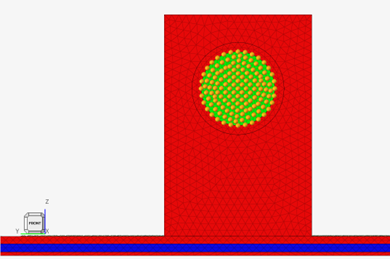
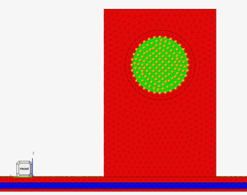
The finite element mesh contains of non-design solid (red), non-design solid with
thermal loading (yellow), non-design fluid (green) and the design space (blue),
which is a layer between upper and lower plate.Figure 1. Model Figure 2. Design Space
The finite element model representing the designable and non-designable material is
imported into HyperMesh. Appropriate properties,
boundary conditions, loads, and optimization parameters are defined and the OptiStruct software determines the optimal cooling
channel.
The following exercises are included:
Import the model into HyperMesh.
Set up the design and solid material.
Set up the optimization.
View the results in HyperView.
Launch HyperMesh
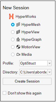
Launch HyperMesh.
In the New Session window, select HyperMesh from the list of tools.
For Profile, select OptiStruct.
Click Create Session.
Figure 3. Create New Session This loads the user profile, including the appropriate template, menus,
and functionalities of HyperMesh relevant for
generating models for OptiStruct.
Open the Model File
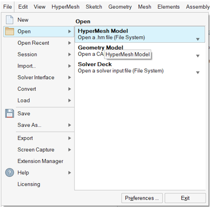
On the menu bar, select File > Open > HyperMesh Model.
Navigate to and select the Battery_pack_base.hm file saved in your
working directory.
Click Open.
The Battery_pack_base.hm database is loaded into the current
HyperMesh session, replacing any existing
data.Figure 4. Model Import Options
Tip: Alternatively, you can drag and drop the file onto the
viewport from the file browser window.
Set Up the Model
Apply Heat Flux
In the Model Browser, double-click
Components to open the Components Browser.
Right-click on the PSOLID_4 component and select
Isolate.
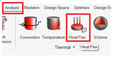
From the menu bar, open the Analyze ribbon.
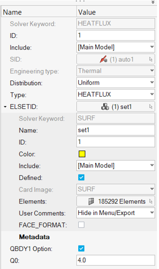
On the ribbon, select Heat Flux.
Figure 5. Select Heat Flux Load
For ELSETID, select the hamburger menu and
click Create.
For Name, accept the default Set 1.
Select elements by faces and choose the front faces of
the PSOLID_4 component.
For QBDY1 Option, ensure Q0 is set to 4.0.
Click
Close.
Figure 6. Choose Surface for Heat Flux Load
Create Inlet Node Set
Un-isolate all other parts.
In the Model Browser, right-click and select
Create > Set.
For Name, enter inlet.
For Card Image, select SET_GRID.
For Entities, select the nodes as shown in Figure 7.
Figure 7. Selection of Inlet Nodes
Figure 8. Create Inlet Node Set
Click
Close.
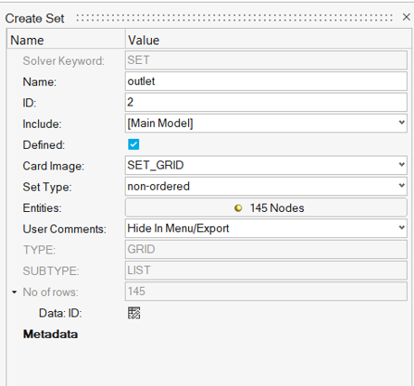
Create Outlet Node Set
In the Model Browser, right-click and select
Create > Set.
For Name, enter outlet.
For Card Image, select SET_GRID.
For Entities, select the nodes as shown in Figure 9.
Figure 9. Selection of Outlet Nodes
Figure 10. Create Outlet Node Set
Click
Close.
Assign Thermal Boundary Condition
In the Model Browser, right-click and select
Create > Load Collector.
A default load collector displays in the Entity Editor.
For Name, enter loadcol1.
Click
Close.
From the menu bar, open the Analyze ribbon.
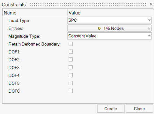
On the ribbon, click Constraints.
Figure 11. Assign Thermal Boundary
For Entities, select Nodes.
Select the nodes of the inlet faces.
Clear the check boxes for DOF1,
DOF2, DOF3,
DOF4, DOF5, and
DOF6.
Click Create and Close.
Create Inlet Pressure and Outlet Pressure
In the Model Browser, right-click and select
Create > Load Collector.
A default load collector displays in the Entity Editor.
For Name, enter loadcol2.
Click
Close.
In the Model Browser, right-click and select
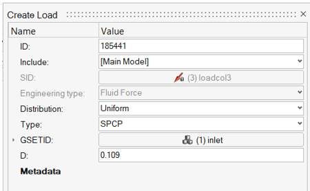
Create > Load.
For Load Type, select SPCP.
For GSETID, select Unspecified > Set > inlet.
For D, enter 0.109.
Click
Close.
Figure 12. Create Inlet Pressure
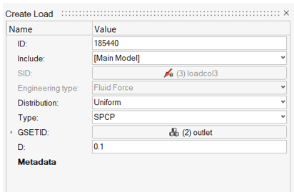
Similarly, create the outlet pressure under the same load collector. In the
Model Browser, right-click and select Create > Load.
For Load Type, select SPCP.
For GSETID, select Unspecified > Set > outlet.
For D, enter 0.1.
Click
Close.
Figure 13. Create Outlet Pressure
Create Subcase
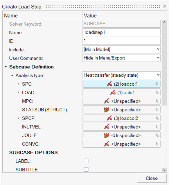
In the Model Browser, right-click and select
Create > Load Step.
For Name, enter loadstep1.
For Analysis type, select Heat Transfer (Steady
State).
In the Select Loadcol dialog for SPC, select
loadcol_1.
For LOAD, select auto_1.
For SPCP, select loadcol_2.
Click
Close.
Figure 14. Create Load Step
Set Up the Optimization
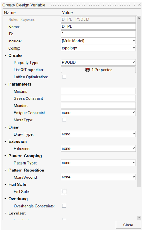
Create Topology Design Space
From the menu bar, open the Optimize ribbon.
On the ribbon, select Topology.
For Name, enter DTPL.
For Property Type, select PSOLID.
For List Of Properties, select property PSOLID_3.
Figure 15. Create Design Variable
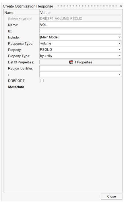
Create Responses
From the menu bar, open the Optimize ribbon.
On the ribbon, select Responses.
For Name, enter VOL.
For Response Type, select volume.
For Property, select PSOLID.
For Property Type, select by entity.
For List Of Properties, select property PSOLID_3.
Click
Close.
Figure 16. Create Optimization Responses
Similarly, create another response and name it
tcomp.
For Response Type, select Thermal compliance.
Click
Close.
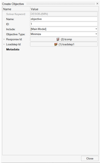
Create Objective
From the menu bar, open the Optimize ribbon.
On the ribbon, select Objectives.
For Objective Type, select Minimize.
For Response Id, click Optimization Response > tcomp.
For Loadstep Id, click Optimization Response > loadstep1.
Click
Close.
Figure 17. Create Objective
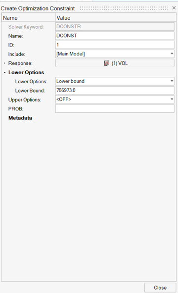
Create Constraints
From the menu bar, open the Optimize ribbon.
On the ribbon, select Constraints.
For Name, enter DCONST.
For Response, click Optimization Response > VOL.
For Lower Options, select Lower Bound and enter 756973
in the text box.
Click
Close.
Figure 18. Create Constraints
Submit the Job
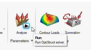
Run OptiStruct.
From the Analyze ribbon, click Run OptiStruct
Solver.
Figure 19. Select Run OptiStruct Solver
Select the directory where you want to write the OptiStruct model file.
For File name, enter battery_pack.
The .fem filename extension is the recommended extension
for Bulk Data Format input decks.
Click Save.
Click Export.
For export options, toggle all.
For run options, toggle optimization.
For memory options, toggle memory default.
In the Altair Compute Console, click
Run.
If the job is successful, an "OptiStruct Job Completed" message appears
in the Compute Console Solver View Message Log. New results
files are in the directory where the model file was written. The
battery_pack.out file is a good
place to look for error messages that could help debug the input deck if any
errors are present.
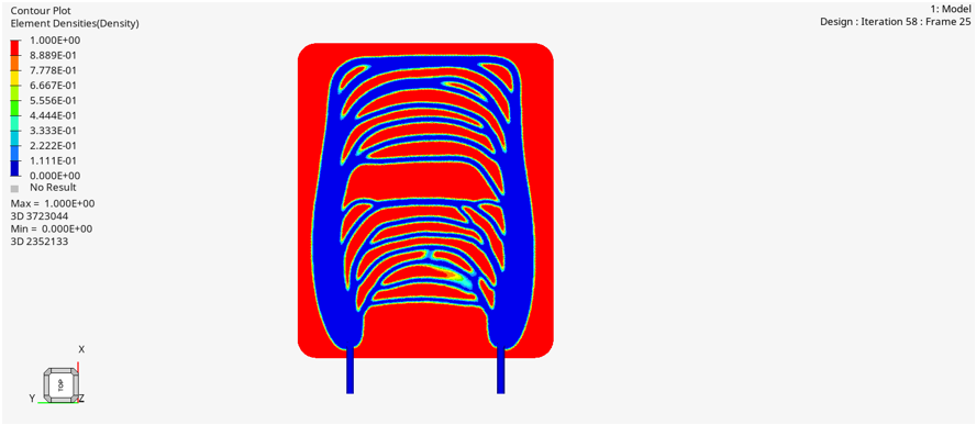
View Contour Plot
Launch HyperView and open the result file.
Click Contour.
Figure 20.
For Result type, select Element Densities (s) from the
first pull-down menu.
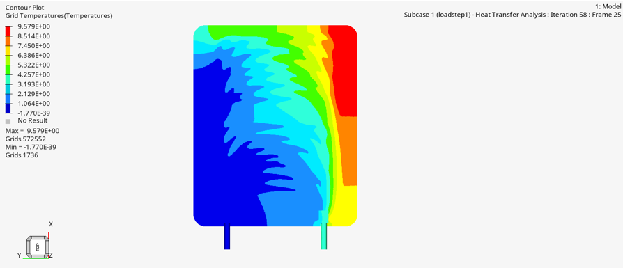
Figure 21. Element Densities Contour Plot Figure 22. Grid Temperature Contour Plot
1 Dienemann, R., Schewe, F. & Elham, A. Industrial
application of topology optimization for forced convection based on
Darcy flow. Struct Multidisc Optim 65, 265 (2022). https://doi.org/10.1007/s00158-022-03328-4

 Heat Flux.
 and
click Create.
and
click Create.

 Constraints.