OS-HM-T: 10010 Design Concept for a Structural Clip
Tutorial Level: Intermediate In this tutorial, a topology optimization on a model is performed to create a new topology
for the structure, removing any unnecessary material. The resulting structure is lighter and
satisfies all design constraints.
The topology optimization technique yields a new design and optimal material
distribution. Topology optimization allows designers to start with a design that
already has the advantage of optimal material distribution and is ready for fine
tuning with shape or size optimization.
Before you begin, copy the file(s) used in this tutorial to your
working directory.
The optimization problem for this tutorial is stated as:
Objective
Minimize volume fraction.
Constraints
Translation in the y-axis for node A < 0.07 mm.
Translation in the y-axis at node B > -0.07 mm.
Design Variables
The density of each element in the design space.
The following exercises are included:
Set up the model in HyperMesh.
Analyze the baseline model.
Set up the optimization.
Post-process size optimization results.
Launch HyperMesh
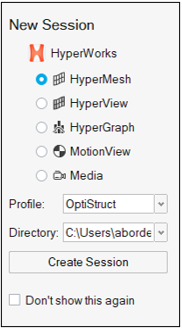
Launch HyperMesh.
In the New Session window, select HyperMesh from the list of tools.
For Profile, select OptiStruct.
Click Create Session.
Figure 1. Create New Session This loads the user profile, including the appropriate template, menus,
and functionalities of HyperMesh relevant for
generating models for OptiStruct.
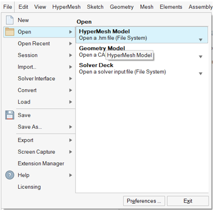
Open the Model File
On the menu bar, select File > Open > HyperMesh Model.
Navigate to and select the cclip.hm file saved in your
working directory.
Click Open.
The cclip.hm database is loaded into the current
HyperMesh session, replacing any existing
data.Figure 2. Model Import Options
Tip: Alternatively, you can drag and drop the file onto the
viewport from the file browser window.
Set Up the Model
Create Materials and Properties for the Components
Properties and materials can be created from within the Component editor.
In the Model Browser, double-click on
Components.
Tip: Alternatively, you can right-click on
Components and click
Open.
Select the component comp_shell.
In the Entity Editor, right click on
Property and select Create.
This creates and assigns the property to the selected
Component.
In the embedded Entity Editor, for Name, enter
prop_shell.
For Card Image, select PSHELL.
Click the T (thickness) field and accept the default
value of 1.0 by pressing Enter.
Right-click on Material and select
Create.
This creates and assigns the material to the selected
component/property.
For Name, enter Steel.
For Card Image, select MAT1.
Click the E field and accept the default value of
2.1E5 by pressing Enter.
Similarly, click the Nu field and accept the default
value of 0.3.
For RHO, enter 7.9E-9.
Click Close.
Close the Entity Editor.
Create Load Collectors
Next, create two load collectors (Constraints and Forces) and assign each a
color.
In the Model Browser, right-click and select
Create > Load Collector.
For Name, enter Forces.
Click Color and
select a color from the color palette.
Click
Close.
Using the same method, create a second load collector named
Constraints.
The Constraints load collector is set as Current as it was created last.
The SPCs created next are set into the Constraints load collector.
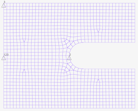
Create Constraints
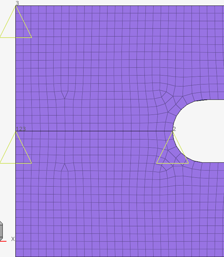
For the three nodes that show constraints in Figure 3, you need to create the SPC constraints and assign them to the Constraints load
collector.Figure 3. Nodes Showing Constraints
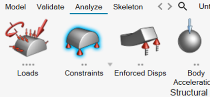
From the Analyze ribbon, click Constraints.
Figure 4. Constraints Tool
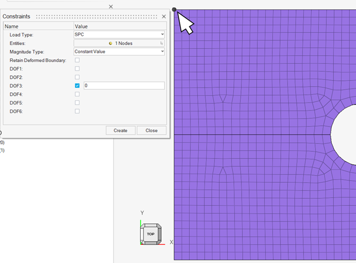
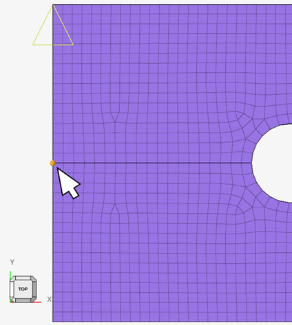
Orient the model to the TOP view.
Select the upper left node and click .
Deselect all DOF check boxes except for DOF3.
For DOF3, accept the default value of 0.
Figure 5. DOF3 Active on Upper Left Node
Tip: To deselect a node, hold Shift and
left-click on it, or left-click + drag a box around it.
For Enties, click Nodes to select another node.
Select the node at the halfway point on the left edge of the part and click
.
Figure 6. Left Middle Node Selection for DOFs 1, 2, 3
Select the DOF1, DOF2, and
DOF3 check boxes.
Accept all default values of 0.
Click Create.
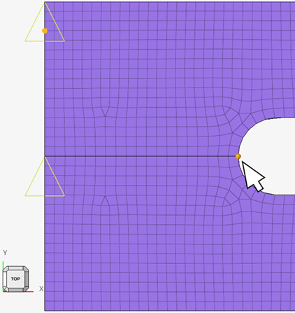
Repeat from step 6 to select the node at the left of the slot radius.
Figure 7. Middle Node on Radius Selection for DOF 2
Select the DOF2 check box and accept the default value
of 0.
Click Create.
Click Close.
Tip: To increase the size of the spc markers: click File > Preferences. Under HyperMesh, click
Appearance. For Boundary conditions, increase the
Size value.
To see the DOF labels, activate
Labels for Boundary Conditions and
Show load handle for Loads.
Figure 8. Boundary Conditions Applied to C-clip
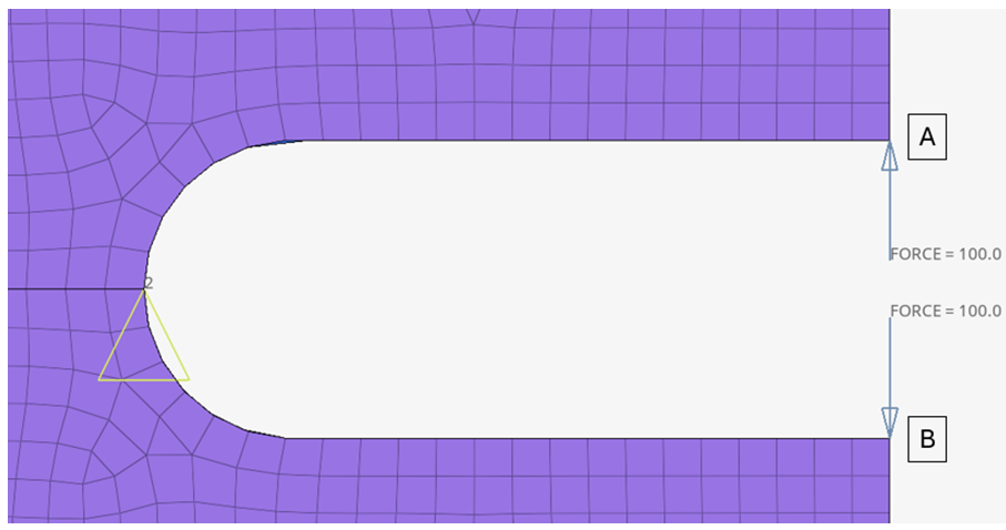
Create Forces
In this step, load the structure with two opposing forces of 100.0 N at the opposite
tips of the opening of the c-clip.
In the Model Browser, double-click on Load
Collectors.
Tip: Alternatively, you can right-click on Load
Collectors and click Open.
Right-click Forces and select Make
Current.
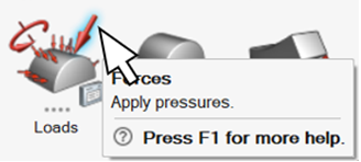
On the Analyze ribbon, Loads tool group, select
Forces.
Figure 9. Forces Tool
Orient the model to the TOP view.
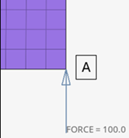
Select the node at the right end, top edge of the slot (location A in Figure 10).
Click .
For Magnitude, enter 100.0.
For Direction, enter X = 0, Y =
1, and Z = 0.
Click Create.
An arrow pointing upward appears at the selected node.
Click Nodes to select another node.
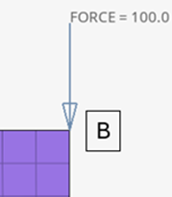
Select the node on the right end, bottom edge of the slot (location B in Figure 10).
Click .
For Magnitude, enter -100.0.
For Direction, verify the values are X = 0, Y =
1, and Z = 0.
Click Create.
An arrow pointing downward appears at the selected node.
Click
Close.
Tip: To increase the size of the load arrows: click File > Preferences. Under HyperMesh, click
Appearance. For Loads, increase the
Uniform value.
Figure 10. Opposing Forces Created at Opening of C-clip
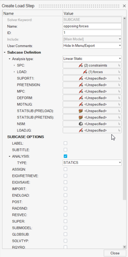
Create Load Cases
The last step in establishing boundary conditions is the creation of a load step.
In the Model Browser, right-click and select
Create > Load Step.
For Name, enter opposing forces.
For Analysis type, select Linear Static.
For SPC, click Unspecified and select the search tool.
Select Constraints from the list.
Similarly, for LOAD, select Forces.
Figure 11. Load Step Defined
Click
Close.
Analyze the Baseline Model
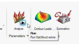
Run the Analysis
A linear static analysis of this C-clip is performed prior to the definition of the
optimization process. An analysis identifies the responses of the structure before
optimization to ensure that constraints defined for the optimization are
reasonable.
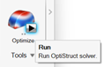
From the Analyze ribbon, click Run OptiStruct
Solver.
Figure 12. Select Run OptiStruct Solver
Select the directory where you want to write the OptiStruct model file.
For File name, enter cclip.
The .fem filename extension is the recommended extension
for Bulk Data Format input decks.
Click Save.
For export options, toggle all.
Click Export.
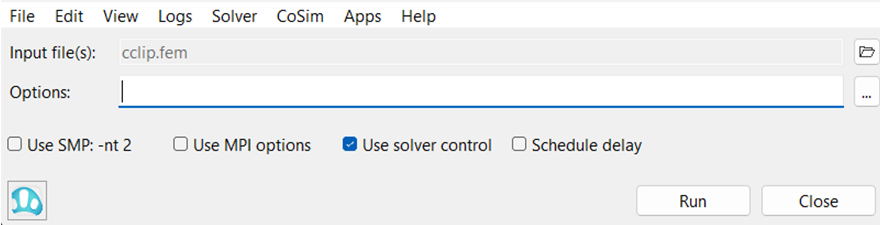
The Compute Console opens with cclip.fem as the
Input File.Figure 13. Altair Compute Console
Click Run.
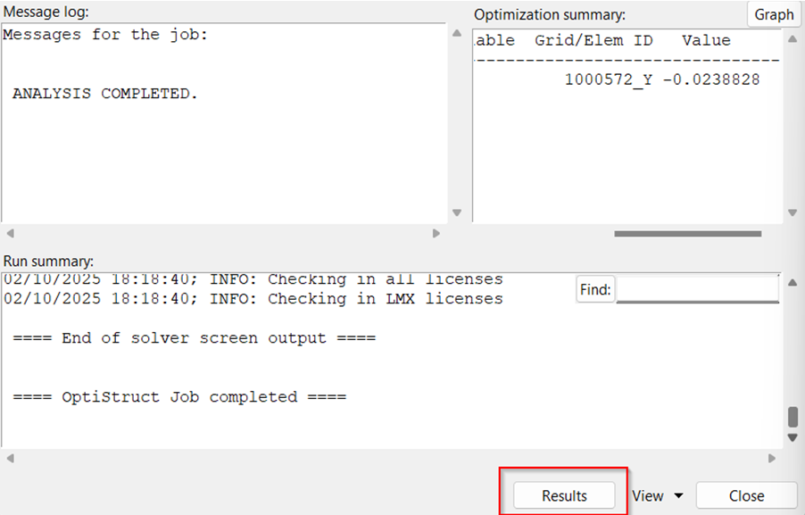
Upon successful completion of the analysis, the message ANALYSIS
COMPLETED appears in the Message log window.
View Displacement Contour
From the Compute Console, click Results to launch the
cclip.mvwresults file in HyperView.
From the menu bar, select File > Exit to close HyperView.
In the Save Session? dialog, click
No.
In the Compute Console Solver View window, click
Close.
In the Compute Console, click Close.
Set Up the Optimization
The finite element model, consisting of shell elements, element properties, material
properties, and loads and boundary conditions has been defined. Now a topology
optimization is performed with the goal of minimizing the amount of material used.
Typically, removing the material in an existing volume with the same loads and
boundary conditions makes the model less stiff and more prone to deformation.
Therefore, you need to track the displacements (which represent the stiffness of the
structure) and constrain the optimization process such that the least material
necessary is used and overall stiffness is also achieved.
The forces in the structure are applied on the outer nodes of the opening of the
clip, making those two nodes critical locations in the mesh where the maximum
displacement is likely to occur. In this tutorial, a displacement constraint is
applied on the nodes so that they do not displace more than 0.07 in the y-axis.
Create the Topology Design Variables
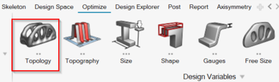
In HyperMesh, open the
Optimize ribbon.
Click Topology.
Figure 17. Topology Tool
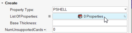
For Property Type, select PSHELL.
For List of Properties, click 0 Properties > to open Advanced Selection.
Figure 18. List of Properties
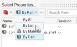
Change the selection type to By List and select
prop_shell.
Figure 19. Select By List
Click OK.
Click
Close.
Create a Volume Response
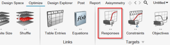
On the Optimize ribbon, click Responses.
Figure 20. Responses Tool
For Name, enter volfrac.
For Response Type, select volumefrac.
Click
Close.
Create a Displacement Response
To create a displacement as a response, supply a name for the response, set the
response type to displacement, select the node for the response, and select the type
of displacement (DOF).
On the Optimize ribbon, click Responses.
For Name, enter upper-disp.
For Response Type, select static displacement.
For List of Nodes, click 0 Nodes.
Select the node at the upper opening of the c-clip (labeled A in Figure 21).
Figure 21. Upper Opening of C-clip
Click .
From the drop-down menu, select dof2.
Click
Close.
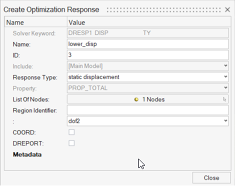
On the Optimize ribbon, click Responses.
For Name, enter lower-disp.
For Response Type, select static displacement.
For List of Nodes, click 0 Nodes.
Select the node at the lower opening of the c-clip (labeled B in Figure 22).
Figure 22. Lower Opening of C-clip
From the drop-down menu, select dof2.
Figure 23. Optimization Response
Click
Close.
Create Constraints on Displacement Responses
In this step, the upper and lower bound constraint criteria for this analysis are
set.
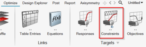
On the Optimize ribbon, click Constraints.
Figure 24. Constraints Tool
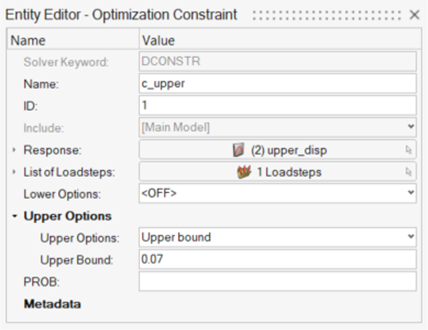
For Name, enter c_upper.
For Response, click Unspecified and select the search tool.
Select upper-disp from the list.
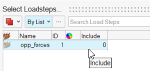
For List of Loadsteps, click 0 Loadsteps > to open Advanced Selection.
Select opposing forces from the list.
Click OK.
Figure 25. Select opposing forces Loadstep
For Upper Options, select Upper bound.
For Upper Bound, enter 0.07.
Figure 26. Optimization Constraint c_upper
Click
Close.
On the Optimize ribbon, click Constraints.
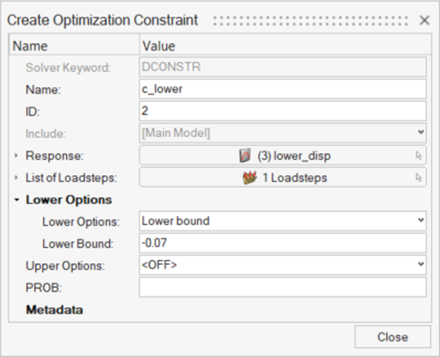
For name, enter c_lower.
For Response, click Unspecified and select the search tool.
Select lower-disp from the list.
For List of Loadsteps, click 0 Loadsteps > to open Advanced Selection.
Select opposing forces from the list.
Click OK.
For Lower Options, select Lower bound.
For Lower Bound, enter -0.07.
Figure 27. Optimization Constraint c-lower
Click
Close.
Define the Objective Function
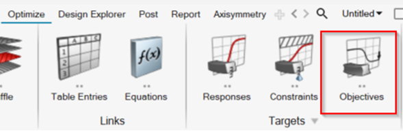
On the Optimize ribbon, select Objectives.
Figure 28. Objectives Tool
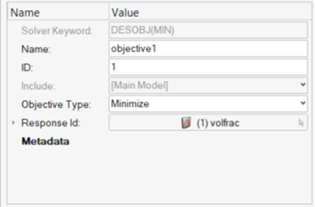
Verify that Objective Type is set to Minimize.
For Response Id, click Unspecified and select the search tool.
Select volfrac.
Figure 29. Objective Definition
Click
Close.
Run the Optimization
From the Optimize tool, click Run.
Figure 30. Run Optimization
Select the directory where you want to write the OptiStruct model file.
For File name, enter cclip_complete.
The .fem filename extension is the recommended extension
for Bulk Data Format input decks.
Click Save.
For Export, select All.
Click Export.
In the Altair Compute Console, click
Run.
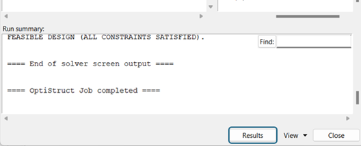
If the job is successful, the following message appears in the window:
OPTIMIZATION HAS CONVERGED.
FEASIBLE DESIGN (ALL CONSTRAINTS SATISFIED).
New results files are seen in the directory where the model file was
written. The cclip_complete.out file is a
good place to look for error messages that could help debug the input deck if
any errors are present.
The following default files are written to your run directory:
cclip_complete_des.h3d
HyperView binary results file
containing the iso surface.
cclip_complete_s1.h3d
HyperView binary results file
containing the displacement and stress results.
cclip_complete.mvw
Contains the design results and the displacement and stress
results from the *_des.h3d and
*_s1.h3d files.
cclip_complete_hist.mvw
Contains the iteration history of the objective, constraints,
and the design variables. It can be used to plot curves in
HyperGraph, HyperView, and MotionView.
cclip_complete.out
OptiStruct output file containing
specific information on the file setup, the setup of the
optimization problem, estimates for the amount of RAM and disk
space required for the run, information for all optimization
iterations, and compute time information. Review this file for
warnings and errors that are flagged from processing the
cclip_complete.fem file.
cclip_complete.sh
Shape file for the final iteration. It contains the material
density, void size parameters, and void orientation angle for
each element in the analysis. This file can be used to restart a
run.
cclip_complete.hgdata
HyperGraph file containing data for
the objective function, percent constraint violations, and
constraint for each iteration.
cclip_complete.oss
OSSmooth file with a default density threshold of 0.3. You can
edit the parameters in the file to obtain the desired
results.
cclip_complete.stat
Contains information about the CPU time used for the complete
run and also the break-up of the CPU time for reading the input
deck, assembly, analysis, convergence, and so on.
Post-process the Results
OptiStruct provides element density
information for all iterations, and also gives displacement and Von Mises stress
results (linear static analysis) for the starting and last iterations. This section
describes how to view those results in HyperView.
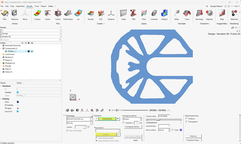
View an Iso Value Plot of Element Densities
From the Compute Console Solver View, click
Results.
Figure 31. View Results
The cclip_complete.mvw file launches in HyperView. This file contains two pages of results:
Page 1 - cclip_complete_des.h3d: Optimization
history results (element density).
Page 2 - cclip_complete_s1.h3d: Subcase 1 results;
initial and final (displacement stress).
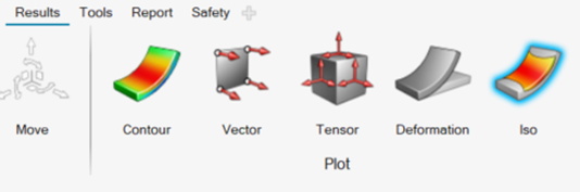
On the Results ribbon, click Iso.
Figure 32. Iso Tool
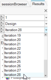
In the Results tab, select the last iteration from the drop-down menu.
Figure 33. Select Last Iteration
Click Apply.
Orient the model to TOP view.
Tip: If the color of the iso surface is difficult to see, go to the
Results tab, expand
Components, and click on the color indicator to
select a different color from the pallet.
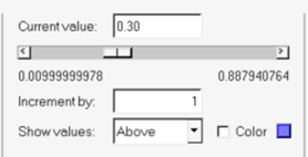
For Current Value, enter 0.3.
Figure 34. Iso Value Slider with Setting 0.3 Figure 35. Results
To change the density threshold, adjust the Current
Value slider.
The iso value updates interactively when you scroll to a new value. Use
this tool to get a better look at the material layout and the load paths from
OptiStruct.
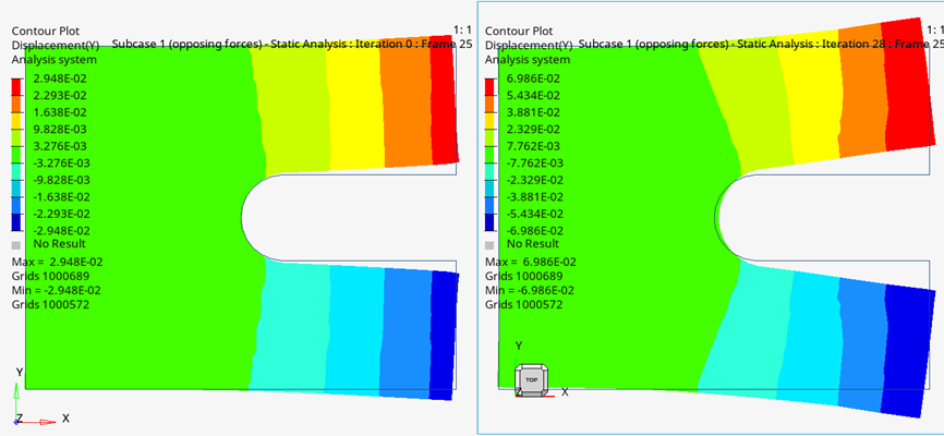
Compare Static Contours
In this step, compare the static contour of the original design to the optimized
material layout.
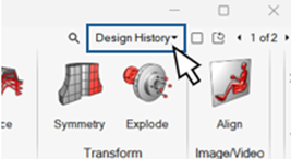
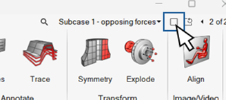
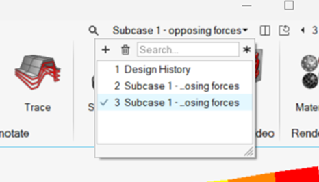
Expand the page selection dialog.
This is located at the top right of the window, near the search tool.Figure 36. Expand Page Selection
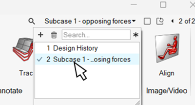
Select Subcase 1 – opposing forces.
Figure 37. Select Subcase 1
Note: If the other pages are not available:
Click File > Import > Model.
Verify the file selected is
cclip_complete_des.h3d.
Click Apply
Click Yes.
Other options should now be available in the page selection
dialog.
Use the Page Layout icon to divide the page into two vertical windows.
Figure 38. Page Layout
Orient the model to TOP view.
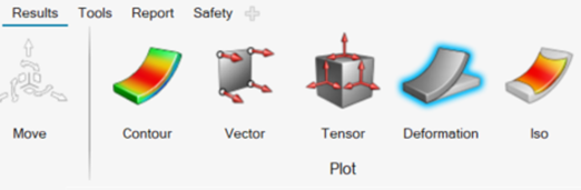
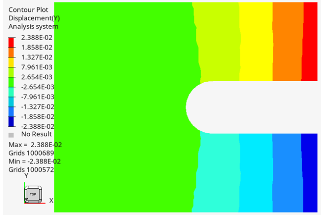
On the Results ribbon, click Contour.
Figure 39. Contour Tool
For Results type, select Displacement.
For the menu below Displacement, select Y.
Click Apply.
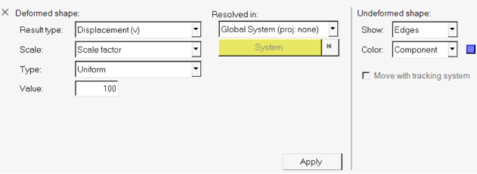
On the Results ribbon, click Deformation.
Figure 40. Deformation Tool
Under Deformed shape, for Value, enter 100.
Under Undeformed shape, for Show, select Edges.
Figure 41. Results Display Settings
Click Apply.
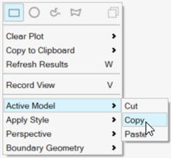
On the Results ribbon, click Contour.
Right-click in the modeling window with the model and
select Active Model > Copy.
Figure 42. Copy Active Model
Right-click in the empty modeling window and select Active Model > Paste.
In the second window, select Iteration 28.
Figure 43. Compare Contour Plots
In the Session Browser, right click on Subcase 1 - opposing forces
2 and select Copy.
Tip: If you do not see the Session Browser, on the menu bar, click View and activate
Session Browser.
Right-click in the Session Browser and select
Paste.
Expand the page selection dialog and select the newly available third
page.
Figure 44. Page Selection
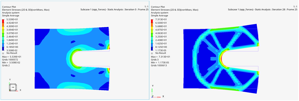
On the new page, click in the left window.
For Results type, select Element Stresses (2D & 3D)
(t).
For Averaging method, select Simple.
Click Apply.
Right-click on the left window and select Apply Style > Current Page > Contour.
The right window now also displays a stress contour.Figure 45. Element Stress Results at Iteration 0 and Iteration 28
These stress results can be used only as reference to help understand
how far the design is from the limits.
Topologic optimization shows a
concept shape and the stress results should be validated during the next
design phases.

 .
.
 search tool.

 to open Advanced Selection.