OS-HM-T: 1300 Direct Frequency Response Analysis of a Flat Plate
Tutorial Level: Beginner This tutorial demonstrates how to import an existing FE model, apply boundary conditions,
and perform a finite element analysis on a flat plate.
Before you begin, copy the file(s) used in this tutorial to your
working directory.
The flat plate is subjected to a frequency-varying unit load excitation using the
direct method. Post-processing is done in HyperView and
HyperGraph to visualize deformations, mode shape
response, and frequency-phase output characteristics.
The following exercises are included:
Set up the problem in HyperMesh
Submit the job
View the results in HyperView and HyperGraph
Launch HyperMesh
Launch HyperMesh.
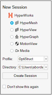
In the New Session window, select HyperMesh from the list of tools.
For Profile, select OptiStruct.
Click Create Session.
Figure 1. Create New Session This loads the user profile, including the appropriate template, menus,
and functionalities of HyperMesh relevant for
generating models for OptiStruct.
Import the Model
On the menu bar, select File > Import > Solver Deck.
In the Import File window, navigate to and select
direct_response_flat_plate_input.fem you saved to your
working directory.
Click Open.
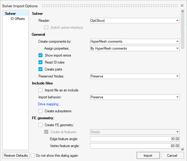
In the Solver Import Options dialog, ensure the Reader is
set to OptiStruct.
Figure 2. Import Base Model in HyperMesh
Accept the default settings and click Import.
Tip: Alternatively, you can drag and drop the file from your file
browser into the application window to open the model file.
Set Up the Model
Apply Loads and Boundary Conditions
In the following steps, the model is constrained at one
edge. A unit vertical load is applied acting upwards in the positive z-direction at
a point on a free edge corner of the plate.
First, the two load collectors (spcs and unit-load) are created.
Click the Model tab to view the Model Browser.
Tip: If you don’t see a Model Browser tab,
you can open it by clicking View > Model Browser on the menu bar.
In the Model Browser, right-click and select
Create > Load Collector.
For Name, enter unit-load.
Click Color and
select a color from the color palette.
Set the Card Image to None.
A new load collector, unit-load, is created.
In the Model Browser, right-click and select
Create > Load Collector.
For Name, enter spcs.
Click Color and select a different color from the
palette.
Set the Card Image to None.
A new load collector, spcs, is created.
Create Constraints
On the Analyze ribbon, select Constraints.
For Entities, select Nodes.
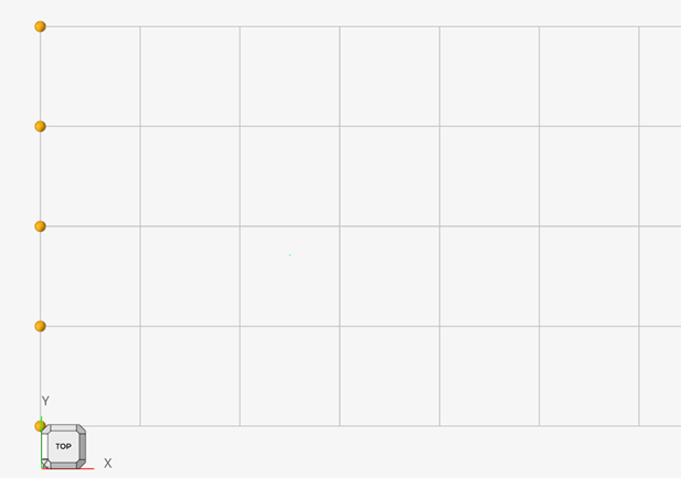
Left click and drag a small box over the left end of the plate (as in Top view)
to select the 5 nodes as shown in Figure 3.
Figure 3. Node selection
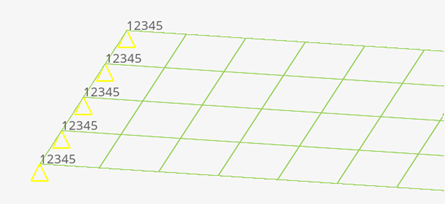
Click to confirm the selection.
In the Constraints dialog, clear the
DOF6 check box and ensure all other DOF check boxes
remain selected.
The selected DOFs are constrained while unselected DOFs are free. DOFs
1, 2, and 3 are x, y and z translation degrees of freedom. DOFs 4, 5, and 6 are
x, y and z rotational degrees of freedom.
Click Create.
The selected nodes are free to rotate about the z-axis since DOF6 was
not selected.
Click
Close.
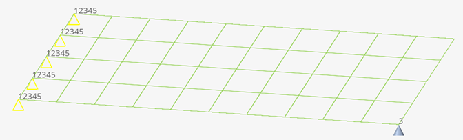
Figure 4. Constrained Nodes
Tip: To increase the size of the spc markers, click File > Preferences. Under HyperMesh, select , Appearance
and increase the Size value for Boundary Conditions. To see the DOF labels,
select Labels for Boundary Condition and
Show load handle for Loads. Click
OK.
Create a Unit Load at a Point on the Flat Plate
In the Model Browser, right-click on the load collector
unit-load and select Make
Current.
On the Analyze ribbon, click Excitations.
For Type, select DAREA.
Next to GSETID, click the hamburger menu and select
Create.
For Entities, verify selection is set to Nodes.
Click Nodes > to open Advanced Selection.
Select By ID.
In the text box, enter, 19 and click
OK.
For Constraint Type, select DOF3 from the extended
entity selection menu.
For Am, enter 20.
Click
Close.
Figure 5. Node Selection for Unit Vertical Load
Create a Frequency Range Table
In the Model Browser, right-click and select
Create > Curve.
A new Curve Editor window opens.
For name, enter tabled1.
In the table, enter the following:
x(1) = 0.0
y(1) =
1.0
x(2) =
1000.0
y(2) =
1.0
Close the window.
In the Model Browser, double-click
Curves.
Select tabled1 to open the card.
For Card Image, select TABLED1 from the drop-down
menu.
This provides a frequency range of 0.0 to 1000.0 with a constant 1.0 over this
range.
Create a Frequency Dependent Dynamic Load
In the Model Browser, right-click and select
Create > Load Step Inputs.
For Name, enter rload2.
For Config Type, select Dynamic Load-Frequency Dependent
from the drop-down list.
For Type, select RLOAD2.
For EXCITEID, click Unspecified.
The load collector appears.
Click the search tool.
Select unit-load from the list of load collectors.
Similarly, for TB, select the tabled1 curve.
The type of excitation can be an applied load (force or moment), an enforced
displacement, velocity or acceleration. The field Type in the RLOAD2 card image
defines the type of load. The type is set to applied load by default.
Click
Close.
Create a Set of Frequencies for the Response Solution
In the Model Browser, right-click and select
Create > Load Collector.
For Name, enter freq1.
Click Color and
select a color from the color palette.
For Card Image, select FREQi from the drop-down
menu.
Select the FREQ1 option and verify the NUMBER_OF_FREQ1
field is set to 1.
If needed, click and enter:
F1 = 20.0
DF = 20.0
NDF
= 49
This provides a set of frequencies beginning
at 20.0 incremented by 20.0 with 49 frequency increments.
Click
Close.
Create a Load Step
In the Model Browser, right-click and select
Create > Load Step.
For Name, enter subcase1.
For Analysis type, select Freq. resp (direct) from the
drop-down menu.
For SPC, open Advanced Selection and choose
spcs from the dialog.
Click OK.
Similarly, for DLOAD, select rload2.
For FREQ, select FREQ1.
This creates an OptiStruct subcase that
references the constraints in the spc load collector and the unit load in the
rload2 load collector with a set of frequencies defined in the freq1 load
collector.
Click
Close.
Create a Set of Nodes for Results Output
In the Model Browser, right-click and select
Create > Set.
For Name, enter SETA.
For Card Image, select Set_Grid from the drop-down menu.
Verify Set Type is set to non-ordered type.
For Entities, click Elements to expand the selection.
Click Nodes.
Select the By ID option and enter 15, 17,
19 in the text box.
Click OK.
Click
Close.
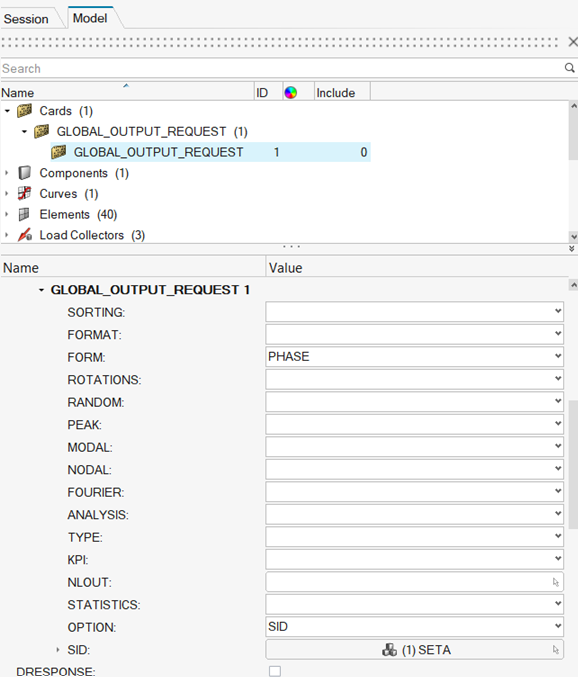
Create a Set of Outputs and Mass Factors for Frequency Response Analysis
In the Model Browser, right-click and select Create > Cards > Output.
In the new window, select the DISPLACEMENT check
box.
In the DISPLACEMENT options, for FORM, select
PHASE.
For OPTION, select SID from the drop-down menu.
For SID, click Unspecified.
For Set, click Unspecified > to open Advanced Selection.
In the dialog, select the By List option and choose
SETA.
Click OK.
(1)SETA now appears in the SID field. This sets the output for only the
nodes in SETA.Figure 6. Output for Nodes in SETA
Click
Close.
In the Model Browser, right-click on
Cards and select Create > More > FORMAT.
In the new window, for number of formats, type 2 and
press Enter.
Next to Data Format_V1, click the table icon.
Select OPTI for 1 and H3D for
2.
Using OPTI generates OptiStructASCII result files like
.disp, .strs, and so on once the run
is complete. These files are used during post-processing.
Click
Close.
In the Model Browser, right-click on
Cards and select Create > PARAM.
Scroll down and select the COUPMASS check box.
For COUPM_V1, select YES.
With this setting, the coupled mass matrix approach for eigenvalue
analysis is used.
Scroll down and select the G check box.
For G_V1, enter 0.06.
This value specifies a uniform structural damping coefficient and is
obtained by multiplying the critical damping ratio by 2.0.
Scroll down and select the WTMASS check box.
For WTM_V1, enter 0.00259.
This factor is used to input all mass entries in weight units. Using
this PARAM multiplies all terms in the mass matrix by this factor.
Click
Close.
In the Model Browser, right-click on
Cards and select Create > OUTPUT.
For KEYWORD, select HGFREQ.
Using HGFREQ results in a frequency output
presentation for HyperGraph.
For FREQ, select ALL to choose all output results for
all frequencies.
Verify number_of_outputs is set to 1.
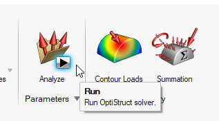
Submit the Job
Run OptiStruct.
From the Analyze ribbon, click Run OptiStruct
Solver.
Figure 7. Select Run OptiStruct Solver
Select the directory where you want to write the OptiStruct model file.
For File name, enter flat_plate_direct_response.
The .fem filename extension is the recommended extension
for Bulk Data Format input decks.
Click Save.
Click Export.
For export options, toggle all.
In the Altair Compute Console, click
Run.
If the job is successful, an "OptiStruct Job Completed" message appears
in the Compute Console Solver View Message Log. New results
files are in the directory where the model file was written. The
flat_plate_direct_response.out file is a good
place to look for error messages that could help debug the input deck if any
errors are present.
The default files written to your
directory are:
flat_plate_direct_response.out
OptiStruct output file containing
specific information on the file setup, the setup of your
optimization problem, estimates for the amount of RAM and disk
space required for the run, information for each of the
optimization iterations, and compute time information. Review
this file for warnings and errors.
flat_plate_direct_response.h3d
HyperView compressed binary results
file.
flat_plate_direct_response.stat
Summary of analysis process, providing CPU information for each
step during process.
Review the Results
This step describes how to view displacement results (.mvw file)
in HyperGraph and also explains the displacement output
(.disp file) from this run. The HyperView results (.h3d file) contains
only the displacement results for the three nodes specified in the node set
output.
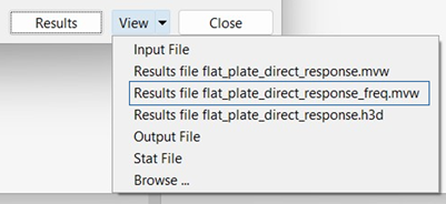
In the Compute Console Solver View window, click View.
From the pull-down list, choose
flat_plate_direct_response_freq.mvw.
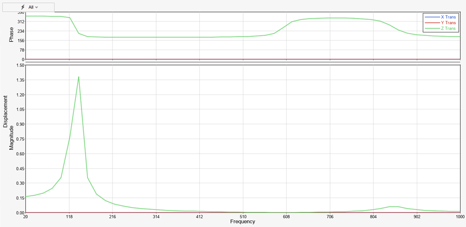
Figure 8. View Menu HyperGraph opens with the
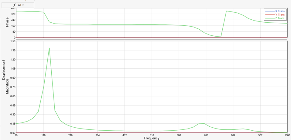
.mvw file loaded. The results for Subcase 1 (subcase 1)
- Displacement of grid 15 are displayed.
There are two sets of results on
this page. The top graph shows Phase Angle verses Frequency. The bottom
graph shows Magnitude versus Frequency.Figure 9. Frequency Response of Node 15
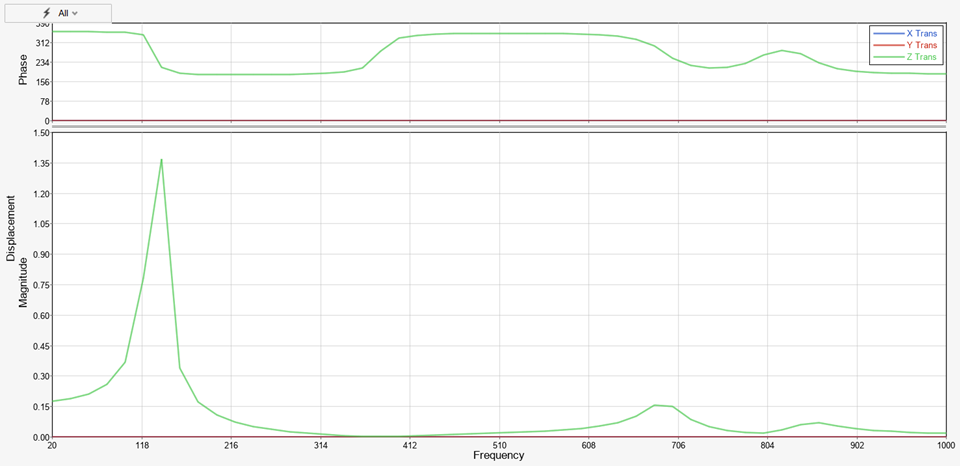
In the Entities list, double click on p2 Subcase 1 (subcase1) -
Displacement of grid 17 to see the graphs for displacement of
grid 17.
Figure 10. Frequency Response of Node 17
Double click on Subcase 1 (subcase1) - Displacement of grid
19 to see the graphs for displacement of grid 19.
Figure 11. Frequency Response of Node 19 This concludes the HyperGraph results
processing.
The first field on the second line shows the iteration number,
the second field shows number of data points, and the third field shows
iteration frequency.
The $DISP [MAG/PHASE] table shows node number,
then x, y and z displacement magnitudes and x, y and z rotation magnitudes.
In the line below the displacement magnitudes for each node, the x, y
and z displacement phase angles and x, y and z rotation phase angles are
listed.

 to confirm the selection.
 to open Advanced Selection.
 search tool.
 and enter:
F1 = 20.0
and enter:
F1 = 20.0