OS-V: 1225 Explicit Analysis on a Dog Bone Model

A tensile test coupon (dog-bone) model is subjected to a dynamic tensile loading and the results of solid and shell elements using different formulations are evaluated.

The goal is to verify the plastic strain results by comparing them with experimental data and Radioss results.

Model Files

Before you begin, copy the file(s) used in this problem to your working directory.

Benchmark Model

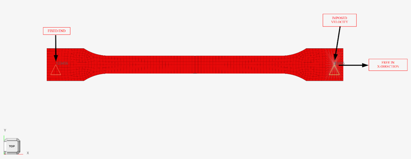
The model represents a tensile test coupon (dog-bone model) as shown in Figure 1. The coupon is extended from one side in the X-direction, while the other side is fixed in all six degrees of freedom using boundary conditions (SPC). The nodes on the right-hand side of the coupon are constrained within a rigid body definition (RBE2). A prescribed velocity of 1m/s in the direction of extension is applied to the main node of the rigid body (SPCD).

The material test data and the engineering stress-strain curves were referred from ^¹. Since experimental stress-strain curves are available, the tabulated material property curve (MATS1) is selected. The formulae in Equation 1 and Equation 2 can be used to determine the true stress versus true strain curve. The plastic part of the curve can then be isolated. This true stress vs plastic true strain curve is used as an input of MATS1.

ε_{t r} = \ln (1 + ε_{e})

σ_{t r} = σ_{e} e x p (ε_{t r})

Where,

$ε_{t r}$: True strain
$ε_{e}$: Engineering strain
$σ_{t r}$: True stress
$σ_{e}$: True strain

The engineering stress can be calculated using σe = F/A0. The force is derived from the rigid body force and the original cross-sectional area is 20.4 mm²

The engineering strain is calculated with εe = Δl/l0. The elongation Δl is measured from two instrumented nodes. The original distance l0 is 80 mm.

Two different element formulations are used in this model and each element formulation has been tested with two different integration types. The following tests were conducted:

CQUAD4 Shell Elements

FULL and BWC integration types are studied
Flanagan-Belytschko Stiffness Form hourglass control is used for BWC

CHEXA Solid Elements

FULL and URI integration types are studied
Puso hourglass control is used for Uniform Reduced Integration (URI)

Material

The specimen is modeled with sheet material using MAT1, which defines the elastic part of the stress strain curve, and MATS1, which defines the plastic part of the curve.

Elastic-plastic Material Properties
Young's modulus: 221.0
Poisson's ratio: 0.3
Density: 7.85E-06
Yield Stress: 0.389674

Plastic Properties

Initial yield point

0.389674

TABLES1 entries for stress strain curve


Strain	Stress
0	389.6743
0.003269061	400.2301
0.006930112	409.5893
0.010444667	418.2536
0.011846377	422.4619
0.012926577	426.8274
0.013648366	433.6494
0.015225465	443.84
0.018589302	452.2541
0.02187438	469.641
0.025339483	483.1056
0.028791504	494.6843
0.032231428	505.9577
0.035658606	515.5831
0.039073858	524.8865
0.042476834	533.055
0.045868261	541.2669
0.049247692	548.5451
0.052615533	555.4787
0.055971597	561.5721
0.059316615	568.0228
0.062650303	574.1739
0.065972157	578.9182
0.069283274	584.1797
0.072583139	588.8521
0.075872187	593.5983
0.079150038	597.5798
0.082417502	602.192
0.085673728	605.6392
0.088919523	609.3784
0.092154789	613.0725
0.095379505	616.5503
0.098593692	619.6955
0.101797797	623.3059
0.104991363	626.2954
0.10817488	629.5215
0.111348321	632.8131
0.114511357	635.3597
0.117664394	637.8515
0.120807432	640.1715
0.123940737	642.7274
0.127064396	645.5801
0.130178021	647.7906
0.133282182	650.4157
0.136376459	652.4523
0.139461486	655.1424
0.142536808	657.36
0.145602624	659.3996
0.148658992	661.2593
0.151706339	663.7797
0.154744129	665.6395
0.15777259	667.1959
0.160792519	670.1453
0.163802712	671.6394
0.166804116	673.6798
0.169796749	676.2103
0.172779798	677.2082
0.175754158	678.6314
0.17871969	680.051
0.181676645	681.9008
0.184624849	683.6876
0.187564155	684.9119
0.190494822	686.0692
0.193600271	686.6066
0.196220092	687.8017
0.19941797	689.0229

Results

The analysis demonstrates the behavior of the tabulated MATS1 material’s stress-strain curve under tensile loading conditions. The simulation results of the engineering stress-strain curves align perfectly with the experimental data and the results from Radioss for all element formulations and integration types. The true stress versus true strain curve is directly extracted from an element at the center of the coupon for all the analyses and the results are as follows:

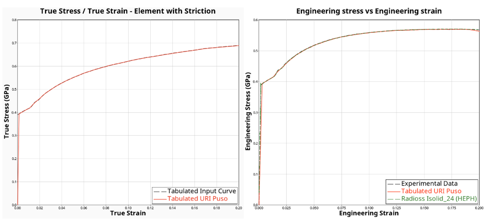
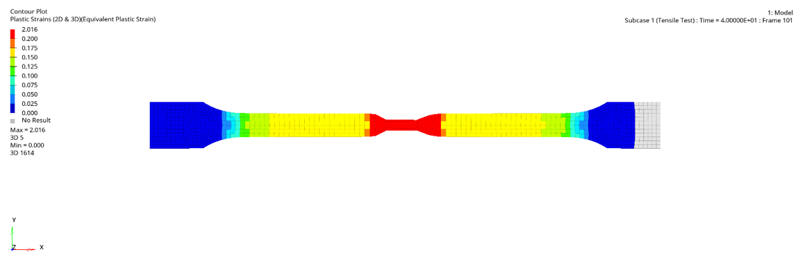
Model with hexahedron elements CHEXA solved using Uniform Reduced Integration (URI) with Puso hourglass control (HGTYP = 2)

Figure 2. Plastic Strain Contour for Solid Element with URI Formulation and Puso HG Control

Figure 3. Comparison of Results using MATS1 for Solid Element with URI Formulation and Puso HG Control

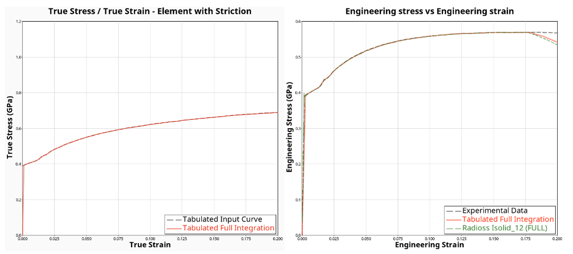
Model with CHEXA elements solved using full integration

Figure 4. Plastic Strain Contour for Solid Element with Full Integration

Figure 5. Comparison of Results using MATS1 for Solid Element with Full Integration

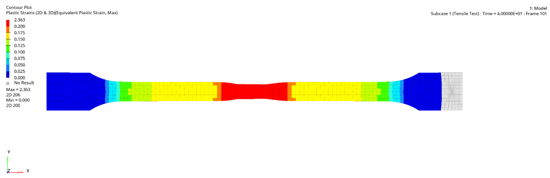
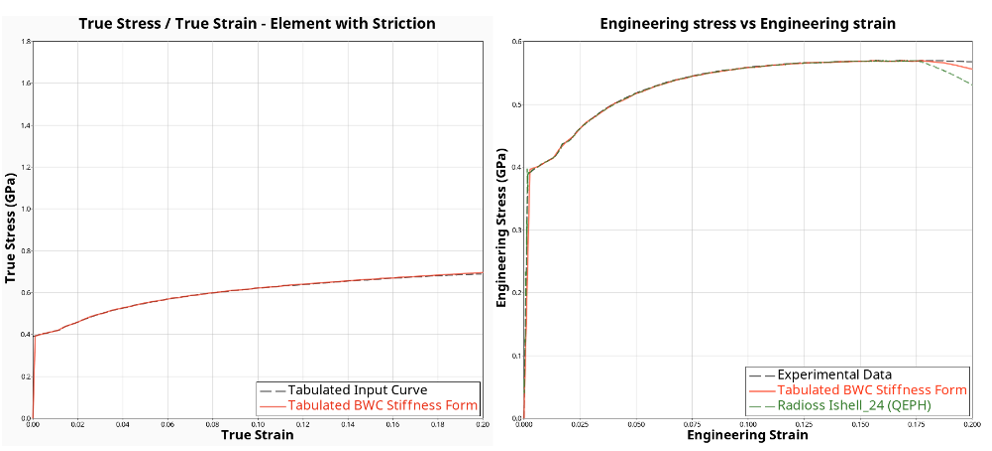
Model with CQUAD4 elements solved using Belytschko-Wong-Chiang (BWC) with Flanagan-Belytschko stiffness form hourglass control (HGTYP = 3)

Figure 6. Plastic Strain Contour for BWC Shell Formulation with Stiffness Hourglass Control

Figure 7. Comparison of Results using MATS1 for Shell BWC Formulation with Stiffness Hourglass Control

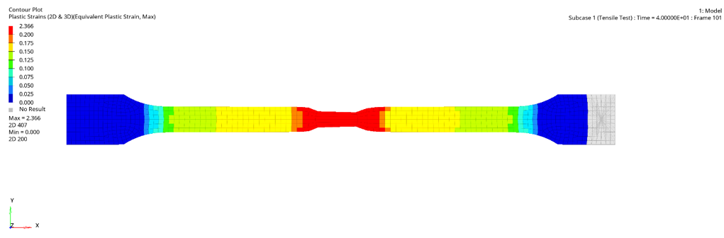
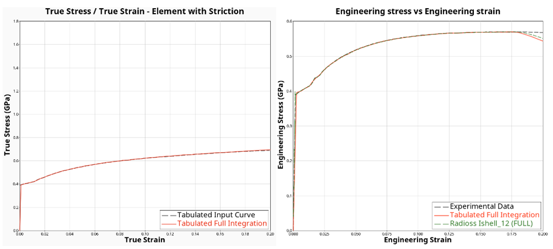
Model with CQUAD4 elements solved using FULL integration

Figure 8. Plastic Strain Contour for Full Integration Shell Formulation

Figure 9. Comparison of Results using MATS1 for Full Integration Shell Formulation

Note: The necking begins at 0.2, so to visualize all elements with plastic strain above this threshold, the second level of the legend is set to 0.2.

Reference

¹ Li, Wenchao & Liao, Fangfang & Zhou, Tianhua & Askes, Harm. (2016). Ductile fracture of Q460 steel: Effects of stress triaxiality and Lode angle. Journal of Constructional Steel Research. 123. 1-17. 10.1016/j.jcsr.2016.04.018.