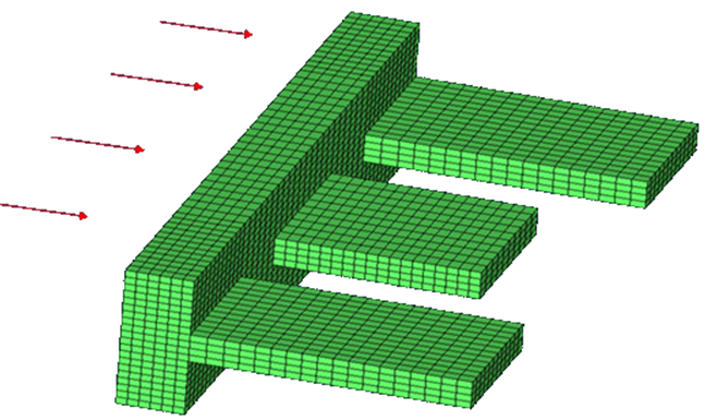
OS-HM-T: 13010 Shape Optimization of Aluminum Fins Based on Heat Transfer
Analysis
Tutorial Level: Advanced In this tutorial, shape optimization on an example of aluminum fins is
performed.
A part of the fins’ base experiences a constant heat flux of q = 8000
W/m2. The temperature of the surrounding air is 283 K, with a
corresponding heat transfer coefficient of H = 40 W/m2 • K. The heat
conduction coefficient is K = 221 W/m • K. The temperature distribution within the
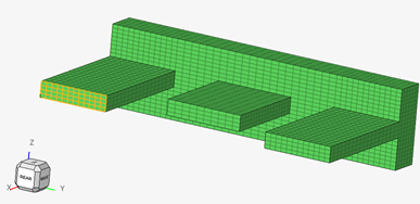
fins is determined by solving the heat conduction and convection load case.Figure 1. Model Overview
Before you begin, copy the file(s) used in this tutorial to your
working directory.
The optimization problem for this tutorial is stated as:
Objective
Minimize the temperature at the center of the base.
Constraints
Volume < 1.0e-5 m2.
Design Variables
Shape design variables.
The following exercises are included:
Set up the shape optimization problem in HyperMesh.
Post-process optimization results in HyperView.
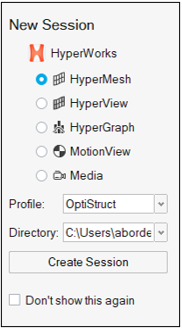
Launch HyperMesh
Launch HyperMesh.
In the New Session window, select HyperMesh from the list of tools.
For Profile, select OptiStruct.
Click Create Session.
Figure 2. Create New Session This loads the user profile, including the appropriate template, menus,
and functionalities of HyperMesh relevant for
generating models for OptiStruct.
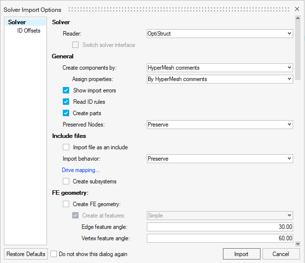
Import the Model
On the menu bar, select File > Import > Solver Deck.
In the Import File window, navigate to and select
fins.fem you saved to your
working directory.
Click Open.
In the Solver Import Options dialog, ensure the Reader is
set to OptiStruct.
Figure 3. Import Base Model in HyperMesh
Accept the default settings and click Import.
Tip: Alternatively, you can drag and drop the file from your file
browser into the application window to open the model file.
Set Up the Optimization
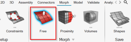
Create Shapes in HyperMorph
The Free morphing function in Morph forms perturbations which are saved as Shapes.
For a more detailed description of the functionality of the Morph page, refer to the
Morph section of the HyperMesh documentation.
Open the Morph ribbon and click
Free.
Figure 4. Free Tool
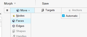
On the guide bar, click Move > Faces.
Figure 5. Guide Bar
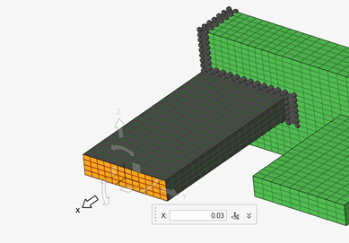
Select the end of one of the fins.
Figure 6. Select End of Fin
Click the arrow pointing normal to the selected element faces
(X-direction).
In the micro-dialog, for X, enter 0.03.
Figure 7. Select X-direction
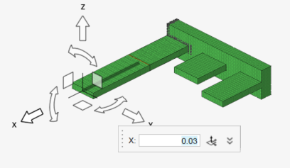
Press Enter.
The fin extends by the value entered in the micro-dialog.Figure 8. Extended Fin
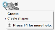
On the Morph ribbon, hover over the Shapes tool and select the
Create satellite icon to save a shape.
Figure 9. Select Create
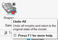
Hover over the Shapes tool and select the Undo All
satellite icon to reset moved elements to their original positions.
Figure 10. Select Undo All
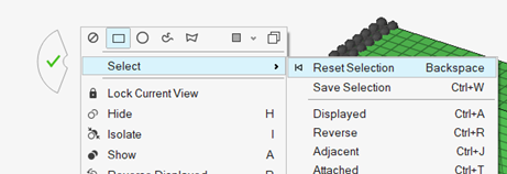
In the modeling window, right-click and select Select > Reset Selection.
Figure 11. Reset Selection
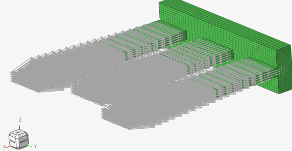
Repeat steps 2 through 9 to create 2 more shapes on the other fins, selecting the end of each fin to
be the facets directly morphed.
Figure 12. Shapes Created on Fins
Note: To control the Shapes display, from the Model Browser you can right-click
on Shapes in the list and select
Hide/Show.
Create Shape Design Variables
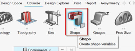
Open the Optimize ribbon and click
Shapes.
Figure 13. Shapes Tool
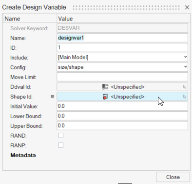
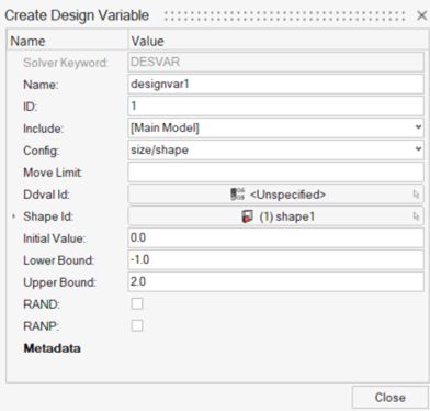
For Shape Id, select Unspecified.
Figure 14. Create Design Variable
Click the Search tool.
Select the first saved shape from the list.
For Initial Value, enter 0.0.
For Lower Bound, enter -1.0.
For Upper Bound, enter 2.0.
Figure 15. Design Variable Defined
Click
Close.
A shape design variable is created from the first saved shape created in
the previous step.
Repeat steps 2 through 8 to create shape design variables from the other two saved shapes.
Create Design Responses
A volume response is created and then defined as the constraint of the optimization
problem. A temperature response is created and then defined as the objective.
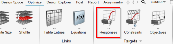
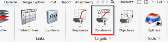
On the Optimize ribbon, Targets tool group, click
Responses.
Figure 16. Responses Tool
For Name, enter volume.
For Response Type, select volume from the drop-down
menu.
Ensure total is selected for Property Type.
Click
Close.
The total volume of the fins is created as the response.
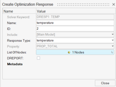
On the ribbon, click Responses.
For Name, enter temperature.
For Response Type, select temperature from the drop-down
menu.
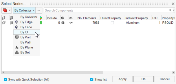
For List of Nodes, click 0 Nodes.
Click to open Advanced Selection.
In the drop-down, choose to select nodes By ID and enter
2450.
Figure 17. Select Nodes by ID
Click OK.
"1 Nodes" is now shown for List of Nodes in the dialog.Figure 18. List of Nodes Shows 1 Node Selected
Click
Close.
The temperature response at node 2450 is created.
Define the Optimization Constraint
On the Optimize ribbon, Targets tool group, click
Constraints.
Figure 19. Constraints Tool
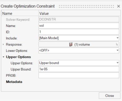
For Name, enter vol.
For Response, click Unspecified.
Click the Search tool.
Select volume from the list of responses.
For Upper Options, select Upper bound from the drop-down
menu.
For Upper Bound, enter 1.0e-5.
Figure 20. Enter Upper Bound
Click
Close.
A volume constraint with the upper bound of 1.0e-5 is
created.
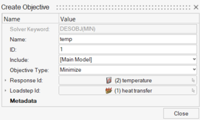
Define the Objective Function
On the Optimize ribbon, Targets tool group, click
Objectives.
For Name, enter temp.
For Objective Type, select Minimize.
For Response Id, click Unspecified.
Click the Search tool and select temperature
from the list of responses.
For Loadstep Id, click Unspecified.
Click the Search tool and select heat
transfer.
Figure 21. temp Objective Parameters
Click
Close.
The objective function of minimizing the temperature at node 2450 is
created.
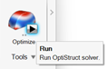
Run the Optimization
From the Optimize tool, click Run.
Figure 22. Run Optimization
Select the directory where you want to write the OptiStruct model file.
For File name, enter fins_opt.
The .fem filename extension is the recommended extension
for Bulk Data Format input decks.
Click Save.
For Export, select All.
Click Export.
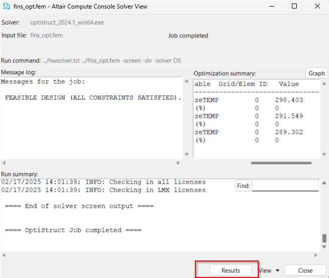
In the Altair Compute Console, click
Run.
If the job is successful, new results files are seen in the directory
where the model file was written. The fins_opt.out file is a good place to look for error messages that could
help debug the input deck if any errors are present.
Post-process the Results
View Contour Plot
In this step, review the contour plot of the temperatures with the optimized shape in
HyperView.
After the "OptiStruct Job completed" message appears in the Run
Summary window, click Results.
This launches HyperView and loads
fins_opt_des.h3d.Figure 23. Launch Results
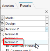
In the Results Browser, select the last iteration.
Figure 24. Show Results Browser Figure 25. Select Last Iteration
On the Results ribbon, Plot tool group, select
Contour.
Figure 26.
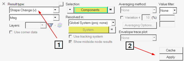
For Result type, select Shape Change (v) and click
Apply.
Figure 27. Select Shape Change (v) Results The optimized shape change contour is displayed.
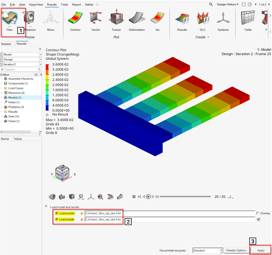
To load the results of the heat transfer loadcase, in the Home tool group,
click Open.
Ensure fins_opt_des.h3d is selected for Load Model and
Load Results.
Click Apply, then click
Yes.
Figure 28. Open Heat Transfer Loadcase
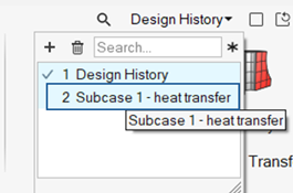
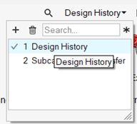
In HyperView, click Design
History to expand the Page Selection
dialog.
Select Subcase 1 - heat transfer.
Figure 29. Select Subcase 1
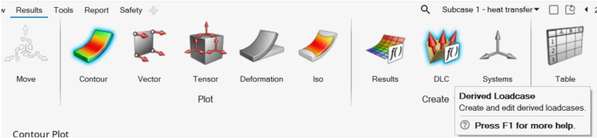
From the Results ribbon, Plot tool group, click
Contour.
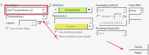
For Result type, select Grid Temperatures (s) and click
Apply.
Figure 30. Select Grid Temperature (s) Results The initial temperature distribution contour in the aluminum fins is
displayed.
In the Results Browser, select the last iteration.
To overlay the optimized temperature results onto the optimized shape results,
switch the Page Selection dialog to the Design
History page.
Figure 31. Page Selection
On the Results ribbon, Create tool group, select
DLC.
Figure 32. DLC Tool
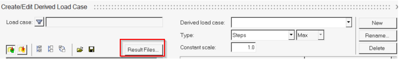
In the Create/Edit Derived Load Case dialog, click
Result Files….
Figure 33. Click Result Files
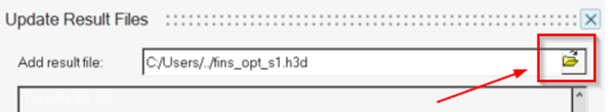
For Add result file, browse to the directory in which the file was run and
select the *__s1.h3d file.
Figure 34. Open File Browser
Click Open.
Click
Close.
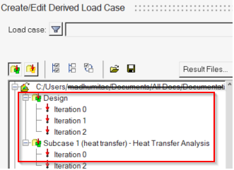
Both the heat transfer results and design results should be visible in
the left window. Figure 35. Results Visible in Left Window
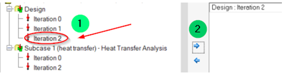
Select the last iteration of the Design results and click to load the result into the derived loadcase list to the right.
Figure 36. Load Result into Derived Loadcase
Repeat step 19 to load the last iteration of the Heat Transfer Analysis results.
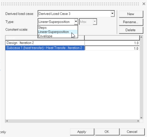
For derived loadcase Type, select
Linear-Superposition.
Figure 37. Select Linear-Superposition
Click OK.
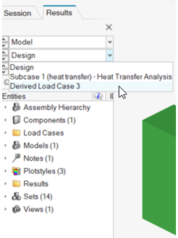
In the Results browser, choose the newly created Derived Load
Case from the drop-down menu.
Figure 38. Select Derived Loadcase
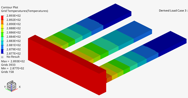
For Result type, select Grid Temperatures (s) and click
Apply.
The contour plot of grid temperature is now applied on top of the
optimized shape. The following plot shows the temperature distributions in the
optimized design. Figure 39. Temperature Distributions in Optimized Design

 Search tool.
 to open Advanced Selection.

 to load the result into the derived loadcase list to the right.