When opening HyperMesh CFD, the Create
Session dialog will appear. Select the Aerodynamics
and Aeroacoustics solution and the
Post-Processing environment.
Note: You may also select the solution and the environment
directly from HMCFD by selectingFile > Solution > Aerodynamics and Aeroacoustics. You may then select the Geometry
Repair environment by selecting from the drop-down to the
right of View.
Figure 1.
Time-Averaged fullData Results
ultraFluidX (uFX) provides its results output in multiple folders which correspond to
the output types. The standard output is placed in the uFX_fullData folder.
Depending on your selected output format, you will find either
.sos or.h3d files within. This
tutorial assumes the Ensight Gold format was selected.
Results Import
From the ribbon selection toolbar (horizontal toolbar), click
Post.
From the horizontal toolbar, click File > Open > Results.
The File Browser opens.
From the File Browser, change the file type to ultraFluidX Results
(.case, .sos,
.h3d).
Navigate to your results directory. Open the
uFX_fullData folder, select
uFX_output.sos and click
Open.
The Reader Options dialog Box opens.Figure 2.
From the Reader Options dialog Box, select
Default Step from the list on the left and set the
Default Step to Last on the drop-down to the right. This
instructs HyperMesh CFD (HMCFD) to load the results from the last timestep
available on the results file to memory.
From the Reader Options dialog, select
Variables from the list on the left and enable the
checkboxes for Compute Q-Criterion, Compute Lambda2, Compute
Vorticity to the right and set the
Gradient variable to
time_avg_velocity. This instructs HMCFD to compute
these field variables using the time-averaged velocity field variable when
computing gradients.
From the Reader Options dialog Box, select
Default Display from the list on the left and make
sure that Cache time-dependent data is
unchecked.
From the Reader Options dialog, press
Import.
The model is imported into HyperMesh CFD.
The Post Browser should now contain a second-level folder
under the name of uFX_output. Right-click on this folder
and click rename. Rename the folder as Standard Output.
If you are unable to see the Post Browser, from the menu
bar, click View, then check Post
Browser.
Calculate Derived Data
From the Post ribbon, click on the Calculate tool.
Figure 3.
The Derived Data Calculator opens.
From the Derived Data Calculator, click on the icon.
The default derived variable list is uploaded.
From the Derived Data Calculator, change the value of velocity_magnitude_inf to
30, that of density_inf to 1.2041, and
that of molecular_viscosity to
1.8194e-05.
Press the save button and save the file as
Aurora_Derived_Data_Calculator.csv.
Note: This step is not required for use of derived data.
Here, the file is being saved for future use with other datasets.
Close the Derived Data Calculator.
Save Boundary Information
From the Post Browser, under Standard Output > Boundary Collections > Flow Boundaries, right click on Body_Exterior_Mirror_Left
and click on Info.
Tip: Use the search tool in the Post
Browser to quickly find the part.
Figure 4.
The Info micro-dialog opens.
Press the save button and save the file as
Body_Exterior_Mirror_Left.csv.
Close the Info micro-dialog.
Repeat steps 1-3 for the following flow boundaries:
From the Post ribbon, click on the Boundary
Groups tool.
Figure 5.
The Boundary Groups guide bar opens.
From the Boundary Groups guide bar, click on the button to open the Advanced
Selection dialog box.
Figure 6.
The Advanced Selection dialog Box opens.
Click on the down arrow of the drop-down menu and select By Boundaries.
Press the checked box icon to select all.
In the search box, type Belt_, then press the empty box icon to unselect the
boundaries with names containing the string: “Belt_”.
Close the Advanced Selection dialog Box. The Display Properties dialog opens in
the Surface Coloring tab. Figure 7: Display Properties dialog – Surface Coloring
tab
Figure 7.
Select Constant from the Display drop-down menu.
Press the green check mark in the Boundary Groups guide
bar.
A new boundary Group is created.
From the Post Browser, find the newly created Boundary
Group in Standard Output > Boundary Collections > Flow Boundaries by using the search utility or by browsing through the tree (it
will be at the bottom).
Right-click on the newly created Boundary Group and click on
Rename. Rename as
Vehicle.
Right-click on Vehicle and click on
Info to save the surface information of the newly
created Boundary Group as Vehicle.csv.
From the Post Browser, right-click on Standard Output > Boundary Collections > Flow Boundaries and click on Delete Empty Boundary
Groups.
Belts
From the Post Browser, group select the remaining flow
boundaries which are not Vehicle, right click and select Create
Boundary Group. Rename the newly created group as
Belts.
From the Post ribbon, click on the
Iso-Surfaces tool.
Figure 8. Figure 9.
The Iso-Surfaces guide bar and
Iso-Function guide panel open.
From the Iso-Function guide panel, set the Iso
Variable to
time_avg_total_pressure_coefficient and the
Iso Value to 0.1, then press
the Calculate button.
The Display Properties micro-dialog opens in the
Surface Coloring tab.
From the Display Properties dialog, Surface
Coloring tab, set the Display value to
constant.
From the Iso-Surfaces guide bar, click on the green check
mark to accept.
From the Post Browser, under Visualizations > Iso-Surfaces, right click on the newly created
Iso-Surface and rename as CpT,
then hide.
Cp+
Repeat Steps 1-5, setting the Iso
Variable to
time_avg_pressure_coefficient, the Iso
Value to 0.5, and renaming the newly
created iso-surface to Cp+.
Cp-
Repeat Steps 1-5, setting the Iso
Variable to
time_avg_pressure_coefficient, the Iso
Value to -0.3, and renaming the newly
created iso-surface to Cp-.
Clips
Y-Clip Vehicle Center | Right
From the Post ribbon, click on the Box
Clip tool.
Figure 10.
The Box Clip guide bar opens.
From the Box Clip guide bar, set the entity selector to
Boundary Groups, then click on the vehicle.
The Vehicle boundary group is highlighted.
From the Box Clip guide bar, click on the
Box button.
Figure 11.
The Box Clip guide panel opens.
Select Outside from the Retain
drop-down.
Press the Fold Frame button to expand the box dimension
fields.
Set Width to 2.0.
Press the Show Move tool button.
From the Move tool, click on the Y
arrow.
Set the Y value to -1 and press
the middle mouse button to accept.
From the Box Clip guide bar, press the
Play button.
The Box Clip is created.
From the Post Browser, under Visualizations > Clips, right click on the newly created Clip and
rename it as Y-Clip Vehicle Center | Right.
Right click on Y-Clip Vehicle Center | Right and click
Hide.
Y-Clip Vehicle Front Axle Center | Right
From the Post ribbon, click on the Scalar
Clip tool.
Figure 12.
The Scalar Clip guide bar opens.
From the Scalar Clip guide bar, set the entity
selector to Boundary Groups, then click
on the vehicle.
Figure 13.
The Vehicle boundary group is highlighted, and the Scalar
Clip guide panel opens..
Select yCrd from the Scalar
drop-down.
Set Range from -2.0 to
-0.82434.
Note: The value of -0.82434 pertains to the y-midpoint of
the front-left tire. You may calculate this value from the data contained in
Wheel_Tire_Front_Left.csv, which was created
following the steps in the Save Boundary Information section.
Select Outside from the Retain
drop-down.
Press the Calculate button.
From the Scalar Clip guide bar, press the green
check mark button to accept.
Rename the new clip as Y-Clip Vehicle Front Axle | Right
and hide the clip.
Note: The value of 0.368879 pertains to the z-midpoint of
the front-left tire. You may calculate this value from the data contained in
Wheel_Tire_Front_Left.csv, which was created
following the steps in the Save Boundary Information section.
Note: The value of 1.03571 pertains to the z-midpoint of
the left mirror. You may calculate this value from the data contained in
Body_Exterior_Mirror_Left.csv, which was created
following the steps in the Save Boundary Information section.
Note: The value of 1.142861 pertains to the z-midpoint of
the front window. You may calculate this value from the data contained in
Body_Exterior_Windshield_Front.csv, which was
created following the steps in the Save Boundary Information section.
Rename the new clip as X-Clip Reference
Iso-Surfaces | Rear and hide the
clip.
From the Post Browser, navigate to Standard Output > Visualizations > Iso-Surfaces and hide all Reference Iso-Surfaces.
Views
Standard
From the View Orientation tool, click on
Left.
Figure 14.
From the bottom left corner of the Viewer, click on the
Store/Recall Views button.
Figure 15.
The Views tool opens.
Rename the newly created View as
Left.
Drag the Views tool to the top left corner of the
screen.
Cycle through the Right, Front, Rear, Top, Bottom, Front-Left, Front-Right,
Rear-Left, Rear-Right, Front-Top-Left, Front-Top-Right, Rear-Top-Left,
Rear-Top-Right, Front-Bottom-Left, Front-Bottom-Right, Rear-Bottom-Left, and
Rear-Bottom-Right orientations. After selecting an orientation, click on
the Capture Current View button in the
Views tool to capture the View
and rename it accordingly.
Front Half
From the Post Browser, under Visualizations > Clips, right click on X-Clip Vehicle Center |
Front and click Show.
Cycle through the Left, Top and Bottom orientations, saving the views and
renaming them accordingly, adding “ | Front” to the end
of each.
From the Post Browser, under Visualizations > Clips, right click on X-Clip Vehicle Center |
Front and click Hide.
Rear Half
From the Post Browser, under Visualizations > Clips, right click on X-Clip Vehicle Center | Rear
and click Show.
Cycle through the Left, Top and Bottom orientations, saving the views and
renaming them accordingly, adding “ | Rear” to the end of
each.
From the Post Browser, under Visualizations > Clips, right click on X-Clip Vehicle Center | Rear
and click Hide.
Wide
From the Post Browser, navigate to Standard Output > Visualizations > Iso-Surfaces and show all Reference Iso-Surfaces.
Cycle through the Left, Right, Front, Rear, Top, Bottom,
Front-Left, Front-Right, Rear-Left, Rear-Right, Front-Top-Left, Front-Top-Right,
Rear-Top-Left, Rear-Top-Right, Front-Bottom-Left, Front-Bottom-Right,
Rear-Bottom-Left, and Rear-Bottom-Right orientations, saving the views and
renaming them accordingly, adding “Wide | ” to the
beginning of each.
Wide | Front Half
From the Post Browser, under Visualizations > Clips, right click on X-Clip Reference Iso-Surfaces |
Front and click Show.
Cycle through the Left, Top and Bottom orientations, saving the views and
renaming them accordingly, adding “Wide |” to the start
and “ | Front” to the end of each.
From the Post Browser, under Visualizations > Clips, right click on X-Clip Reference Iso-Surfaces |
Front and click Hide.
Wide | Rear Half
From the Post Browser, under Visualizations > Clips, right click on X-Clip Reference Iso-Surfaces |
Rear and click Show.
Cycle through the Left, Top and Bottom orientations, saving the views and
renaming them accordingly, adding “Wide |” to the start
and “ | Rear” to the end of each.
From the Post Browser, under Visualizations > Clips, right click on X-Clip Reference Iso-Surfaces |
Rear and click Hide.
From the Post Browser, navigate to Standard Output > Visualizations > Iso-Surfaces and hide all reference Iso-Surfaces.
Image and Video Capture
To capture the image on the viewer, from the menu bar, click File > Screen Capture > Image to File.
To capture a video by cycling through the results frames of the results shown
on the viewer, from the menu bar, click File > Screen Capture > Video to File.
Surface Results
Cp (Time-Averaged)
From the Post Browser, under Boundary Collections > Flow Boundaries, right click on Vehicle and click
Edit.
The Display Properties dialog – Surface
Coloring tab opens.
From the Display Properties dialog – Surface
Coloring tab, set the Display value to
time_avg_pressure_coefficient.
Set the Legend Type to
Global.
Toggle-on the Legend
button.
Set the Legend range from -1 to
1.
Press the Legend button.
Figure 16.
The Legend micro-dialog opens.
From the Legend micro-dialog, click on
Colormap and under Name,
change the value to Cool to Warm (Extended).
From the Legend micro-dialog, click on
Title, type Cp (time-averaged)
in the Title field and check the Horizontal
title check box.
From the Legend micro-dialog, click on
Format. Change the Precision
value to 2 and the Colorbar labels
value to Floating point.
From the Legend micro-dialog, click on
Display. Change the position to Upper
Right Corner by clicking on the Upper Right
Corner button, set the Orientation to
Horizontal, and change the
Length value to 0.2.
From the Display Properties micro-dialog, switch to the
Contour Line Display tab (third from the left on
top).
Figure 17.
From the Display Properties dialog – Contour Line Display
tab, toggle the Display button and set the
Display value to 5.
Set the value of Variable to
time_avg_pressure_coefficient.
Set the Contour Range from -1 to
1 and set Color to
constant.
From the Boundary Groups guide bar, click on the green
check mark to accept.
Cycle through the Left, Top, Bottom, Front, Rear views and capture images for
each.
Cp (time-averaged) – Narrow Range
From the Post Browser, under Boundary Collections > Flow Boundaries, right click on Vehicle and click
Edit.
The Display Properties dialog – Surface Coloring
tab opens.
Set the Legend range from -0.3 to
0.
From the Display Properties micro-dialog, switch to the
Contour Line Display tab (third from the left on
top).
Set the Display value to 7.
Set the Contour Range from -0.3 to
0.
From the Boundary Groups guide bar, click on the
green check mark to
accept.
Cycle through the Rear, Top, Bottom, Front, Rear, Front-Bottom-Right,
Front-Bottom-Left, Rear-Bottom-Right, Rear-Bottom-Left views and
capture images for each.
Cf (Time-Averaged)
From the Post Browser, under Boundary Collections > Flow Boundaries, right click on Vehicle and click
Edit.
The Display Properties dialog – Surface Coloring
tab opens.
From Display Properties dialog – Surface Coloring tab, set
the Display value to
time_avg_skin_friction_coefficient.
Set the Legend Type to
Global.
Set the Legend range from 0 to
0.005.
Press the Legend button.
The Legend micro-dialog opens.
From the Legend micro-dialog, click on
Colormap and under Name,
change the value to Inferno.
From the Legend micro-dialog, click on
Title, type Cf (time-averaged)
in the Title field and check the Horizontal
title check box.
From the Legend micro-dialog, click on
Format. Change the Precision
value to 1 and set the Colorbar
labels value to Exponential.
From the Legend micro-dialog, click on
Display. Change the position to Upper
Right Corner by clicking on the Upper Right Corner button, set
the Orientation to Horizontal, and
change the Length value to
0.2.
From the Display Properties micro-dialog, switch to the
Contour Line Display tab (third from the left on
top).
Toggle-on Display and set the value to
6.
Set the value of Variable to
time_avg_skin_friction_coefficient.
Set the Contour Range from 0 to
0.005, select constant from the Color drop-down, and
set the color to white.
From the Boundary Groups guide bar, click on the
green check mark to
accept.
Cycle through the Rear, Top, Bottom, Front, and Rear views and capture images
for each.
Cf (Time-Averaged) – Narrow Range
From the Post Browser, under Boundary Collections > Flow Boundaries, right click on Vehicle and click
Edit.
The Display Properties dialog – Surface Coloring
tab opens.
Set the Legend range from 0 to
0.003.
From the Display Properties micro-dialog, switch to the
Contour Line Display tab (third from the left on
top).
Set the Display value to 7.
Set the Contour Range from -0 to
0.003.
From the Boundary Groups guide bar, click on the green
check mark to accept.
Cycle through the Rear, Top, Bottom, Front, Rear, Front-Bottom-Right,
Front-Bottom-Left, Rear-Bottom-Right, Rear-Bottom-Left, Top | Front, Bottom |
Front, Top | Rear, and Bottom | Rear views and capture images for each.
Surface Velocity BC
From the Post Browser, under Boundary Collections > Flow Boundaries, right click on Vehicle and click
Edit.
The Display Properties dialog – Surface Coloring
tab opens.
Set the Display value to
velocity.
Set the Legend Type to
Global.
Click on the lightning button of the Legend field to Reset Range.
Press the Legend menu button.
The Legend micro-dialog opens.
From the Legend micro-dialog, click on
Title, type Surface Velocity
BC in the Title field and check the
Horizontal title check box.
From the Legend micro-dialog, click on
Format. Change the Precision
value to 2 and set the Colorbar
labels value to Floating point.
From the Legend micro-dialog, click on
Display. Change the position to Upper
Center by clicking on the Upper Center
button, set the Orientation to
Horizontal, and change the
Length value to 0.3.
From the Legend micro-dialog, click on Colormap, then
check the Scalar based opacity checkbox, and click on the
menu next to it.
Figure 18.
The Scalar Based Opacity dialog opens.
From the Scalar Based Opacity dialog, make sure the
Opacity type is set to
Normalized, and the User defined
range checkbox is checked.
From the Scalar Based Opacity dialog, click on the
Plus button to add a row to the table (there should
now be three) and set the values as shown in the figure above.
Close the Scalar Based Opacity dialog.
From the Display Properties micro-dialog, switch to the
Contour Line Display tab and toggle off the
Display field.
From the Boundary Groups guide bar, click on the green
check mark to accept.
From the Post Browser, under Boundary Collections > Flow Boundaries, right click on Belts and click
Show.
From the Post Browser, under Boundary Collections > Flow Boundaries, right click on Belts and click
Edit.
The Display Properties dialog – Surface
Coloring tab opens.
Set the Display value to
velocity.
Set the Legend Type to
Global.
From the Boundary Groups guide bar, click on the green
check mark to accept.
From the Post ribbon, click on the Surface
Streamlines tool.
Figure 19.
The Surface Streamlines guide bar
opens.
From the Surface Streamlines guide bar, set the selector
type to Boundary Groups, then use the Advanced
Selection tool to select the Vehicle and
Belts boundary groups.
Note: You must close the Advanced
Selection tool for the selection to apply.
From the Surface Streamlines guide bar, click on the
Seeds button. The Seeds
micro-dialog opens.
Figure 20.
From the Seeds micro-dialog, set the Target
point count to 3000.
From the Seeds micro-dialog, click on the hamburger menu
expander.
Figure 21.
The Generation Method micro-dialog
opens.
From the Generation Method micro-dialog, set the
Vector variable to velocity and the
Integration direction to
both.
From the Seeds micro-dialog, click on
Calculate. The Display
Properties dialog – Surface Coloring tab
opens.
From the Display Properties dialog – Surface
Coloring tab, toggle off Display.
From the Display Properties micro-dialog, switch to the
Vector Display tab.
Figure 22.
The Display Properties micro-dialog –
Vector Display tab opens.
From the Display Properties micro-dialog –
Vector Display tab, toggle on the
display button. Set the
Display value to velocity, the
Vector scale factor to
0.1.
Set Color to constant and set the
color to black.
Toggle the Subset button and move the slider all the way
to the left.
Click on the hamburger menu in the Display row to expand
the Vector Specifications micro-dialog.
Figure 23.
From the Vector Specifications micro-dialog, set the
Vector length to
Uniform.
From the Surface Streamlines guide bar, click on the
green check mark to accept.
From the Post Browser, under Standard Output > Visualizations > Surface Streamlines, right click on the newly created Surface
Streamlines and rename as
Vehicle_and_Belts.
Capture an image using the Front-Top-Left view.
From the Post Browser, under Standard Output > Visualizations > Surface Streamlines, right click on Vehicle_and_Belts and click
Hide.
From the Post Browser, under Standard Output > Boundaries > Flow Boundaries, right click on Belts and click
Hide.
From the Post Browser, right click on Legend Manager, then click on Edit.
Figure 24.
The Legend Manager micro-dialog opens.
From the Legend Manager micro-dialog, for the
Legend Variable velocity, toggle off the
Legend.
Press Esc key on the keyboard or right-click on the viewer and swipe left to
exit the Legend Manager micro-dialog.
Surface Streamlines
From the Post Browser, under Boundary Collections > Flow Boundaries, right click on Vehicle and click Edit.
The Display Properties dialog – Surface
Coloring tab opens.
From the Display Properties dialog – Surface
Coloring tab, set the Display value to
constant.
From the Boundary Groups guide bar, click on the green
check mark to accept.
From the Post ribbon, click on the Surface
Streamlines tool.
The Surface Streamlines guide bar
opens.
From the Surface Streamlines guide bar, set the
selector type to Boundary
Groups, then click on any surface of the
Vehicle boundary group to select.
From the Surface Streamlines guide bar, click on the
Seeds button.
The Seeds micro-dialog opens.
From the Seeds micro-dialog, set the Target
point count to 3000.
From the Seeds micro-dialog, click on the hamburger menu
expander.
The Generation Method micro-dialog
opens.
From the Generation Method micro-dialog, set the
Vector variable to time avg wall shear
stress and the Integration direction to
both.
From the Seeds micro-dialog, click on
Calculate.
The Display Properties dialog – Surface
Coloring tab opens.
From Display Properties dialog – Surface
Coloring tab, set the Display value to
time_avg_skin_friction_coefficient.
Press the Display hamburger menu button and set the
Tube radius to 1.
Set the Legend Type to
Global.
Toggle-on the Legend button.
Set the Legend range from 0 to
0.005.
From the Surface Streamlines guide bar, click on the
green check mark to accept.
From the Post Browser, under Standard Output > Visualizations > Surface Streamlines, right click on the newly created Surface
Streamlines and rename as Vehicle.
Cycle through the Rear, Top, Bottom, Front, Rear, Front-Bottom-Right,
Front-Bottom-Left, Rear-Bottom-Right, Rear-Bottom-Left, Top | Front Half, Bottom
| Front Half, Top | Rear, and Bottom | Rear views and capture images for
each.
From the Post Browser, under Standard Output > Visualizations > Surface Streamlines, right click on Vehicle and click
Hide.
Slice Planes
Y Slices
Y-Slice Vehicle Center
Cp (Time-Averaged)
From the Post ribbon, click on the Slice
Planes tool.
Figure 25.
The Slice Planes guide bar opens.
X, Y, and Z Planes are drawn along the centroid of the vehicle.
Figure 26.
Click on the Y-Plane.
Figure 27.
The Slice Plane micro-dialog opens.
From the Slice Plane micro-dialog, check Finite
slice, then expand the micro-dialog by clicking on the
Fold Frame button on the top-right corner and set the
Length to 9 and
Width to 3.
Figure 28.
Press Calculate.
The Display Properties dialog – Surface
Coloring tab opens.
From the Display Properties dialog – Surface
Coloring tab, set the Display value to
time_avg_pressure_coefficient.
Set the Legend range from -1.0 to
1.0
From the Display Properties micro-dialog, switch to the
Contour Line Display tab.
From the Display Properties dialog – Contour
Line Display tab, toggle-on the Display
button.
Set the Display value to
11.
Set the Variable value to
time_avg_pressure_coefficient and the
Contour range to -1.0 to
1.0.
Select constant from the Color drop-down and set the
color to black.
From the Slice Plane guide bar, click on the green check
mark to accept.
From the Post Browser, under Standard Output > Visualizations > Slice Planes, right click on the newly created Slice
Plane and rename to Y-Slice Vehicle
Center.
From the Post Browser, under Standard Output > Boundary Collections > Flow Boundaries, right click on Vehicle and click Edit.
Set transparency to 50% by moving
the transparency slider to the middle position.
From the Boundary Groups guide bar, click on the green check mark to
accept.
From the Post Browser, under Standard Output > Visualizations > Clips, right click on Y-Clip Vehicle Center | Right and click
Show.
Cycle through the Wake | Left , Left | Front, and Wake | Left | Rear views and
capture images for each.
Cp (Time-Averaged, Narrow)
From the Post Browser, under Standard Output > Visualizations > Slice Planes, right click on Y-Slice Vehicle Center and click Edit.
The Display Properties dialog – Surface
Coloring tab opens.
From the Display Properties dialog – Surface Coloring tab, set the Legend range
from -0.3 to 0.
From the Display Properties micro-dialog, switch to the Contour Line Display
tab.
From the Display Properties dialog – Contour Line Display tab, set the Display
value to 7, and the Contour range to -0.3 to 0.
From the Post Browser, under Standard Output > Visualizations > Slice Planes,
right click on Y-Slice Vehicle Center and click Edit.
The Display Properties dialog – Surface Coloring tab opens.
From the Display Properties dialog – Surface Coloring tab, set the Display
value to time_avg_velocity_magnitude_coefficient.
Set the Legend Type to Global.
Toggle-on the Legend button.
Set the Legend range to 0 to
1.2.
Press the Legend hamburger menu button.
The Legend micro-dialog opens.
From the Legend micro-dialog, click on
Colormap and under Name,
change the value to Cool to Warm (Extended).
From the Legend micro-dialog, click on Title, type
Cv (time-averaged) in the
Title field.
From the Legend micro-dialog, click on
Format. Change the Precision
value to 2 and the Colorbar labels
value to Floating point.
From the Legend micro-dialog, click on
Display. Change the position to Upper
Right Corner by clicking on the Upper Right
Corner button, set the Orientation to
Horizontal, and change the
Length value to 0.2.
From the Display Properties micro-dialog, switch to the Contour Line Display
tab.
From the Display Properties dialog – Contour
Line Display tab, toggle-on the Display
button.
Set the Display value to 7.
Set the Variable value to
time_avg_velocity_magnitude_coefficient, and the
Contour range to 0 to
1.2.
Select constant from the Color
drop-down and set the color to black.
From the Slice Plane guide bar, click on the green check
mark to accept.
Cycle through the Wake | Left , Left | Front, and Wake | Left | Rear views and
capture images for each.
Cv (Time-Averaged) + Streamlines
From the Post Browser, under Standard Output > Visualizations > Slice Planes, right click on Y-Slice Vehicle Center and
click Edit.
The Display Properties dialog – Surface
Coloring tab opens.
From the Display Properties micro-dialog, switch to the Contour Line Display
tab.
From the Display Properties dialog – Contour
Line Display tab, toggle-off the Display
button.
From the Post ribbon, click on the Surface Streamlines tool.
From the Surface Streamlines guide bar, set the selector
type to Slice Planes, then click on the Y-Slice
Vehicle Center slice plane.
From the Surface Streamlines guide bar, click on the Seeds button.
The Seeds micro-dialog opens.
From the Seeds micro-dialog, set the Target
point count to 1000.
From the Seeds micro-dialog, click on the hamburger menu expander.
The Generation Method micro-dialog opens.
From the Generation Method micro-dialog, set the
Vector variable to time avg
velocity and the Integration direction to
both.
From the Seeds micro-dialog, click on
Calculate.
The Display Properties dialog – Surface
Coloring tab opens.
From the Display Properties dialog – Surface
Coloring tab, set the Display value to
constant and the color to
black.
Slide the Transparency bar about
70% to the right.
Click on the Display hamburger menu button and set the Tube
radius to 1.
From the Surface Streamlines guide bar, click on the green check mark to
accept.
From the Post Browser, under Standard Output > Visualizations > Surface Streamlines, right click on the newly created Surface
Streamlines and rename to Y-Slice Vehicle
Center.
Cycle through the Wake | Left , Left | Front, and Wake | Left | Rear views and
capture images for each.
From the Post Browser, under Standard Output > Visualizations > Clips, right click on Y-Clip Vehicle Center |
Right and click Hide.
From the Post Browser, under Standard Output > Visualizations > Slice Planes,
right click on Y-Slice Vehicle Center and click Hide.
From the Post Browser, under Standard Output > Visualizations > Surface Streamlines, right click on Y-Slice Vehicle Center and
click Hide.
Y-Slice Front Axle Center
Cp (Time-Averaged)
From the Post ribbon, click on the Slice
Planes tool.
The Slice Plane guide bar opens.
Click on the Y-Plane.
The Slice Plane micro-dialog opens.
From the Slice Plane micro-dialog, check Finite slice, then expand the
micro-dialog by clicking on the Fold Frame button on the top-right corner and
set the Length and Width to 9 and 3 respectively.
From the Slice Plane micro-dialog, click on the Show move tool button, then
click on the Y-Arrow. In the Y field, enter -0.82434, then middle click on the
screen.
From the Post Browser, under Standard Output > Visualizations > Slice Planes,
right click on the newly created Slice Plane and rename to Y-Slice Front Axle
Center.
From the Post Browser, under Standard Output > Visualizations > Clips, right click on Y-Clip Vehicle Front Axle Center |
Right and click Show.
Cycle through the Wake | Left , Left | Front, and Wake | Left | Rear views and
capture images for each.
Cp (Time-Averaged, Narrow)
From the Post Browser, under Standard Output > Visualizations > Slice Planes, right click on Y-Slice Front Axle Center and click Edit.
The Display Properties dialog – Surface
Coloring tab opens.
From the Display Properties dialog – Surface Coloring tab, set the Legend range
from -0.3 to 0.
From the Display Properties micro-dialog, switch to the Contour Line Display
tab.
From the Display Properties dialog – Contour Line Display tab, set the Display
value to 7, and the Contour range to -0.3 to 0.
From the Slice Plane guide bar, click on the green check mark to accept.
Cycle through the Wake | Left , Left | Front, and Wake | Left | Rear views and
capture images for each.
Cv (Time-Averaged)
From the Post Browser, under Standard Output > Visualizations > Slice Planes, right click on Y-Slice Front Axle Center
and click Edit.
The Display Properties dialog – Surface
Coloring tab opens.
From the Display Properties dialog – Surface
Coloring tab, set the Display value to
time_avg_velocity_magnitude_coefficient, and the
Legend range to 0 to 1.2.
From the Display Properties micro-dialog, switch to the Contour Line Display
tab.
Set the Variable value to
time_avg_velocity_magnitude_coefficient, and the
Contour range to 0 to
1.2.
From the Slice Plane guide bar, click on the green check
mark to accept.
Cycle through the Wake | Left , Left | Front, and Wake | Left | Rear views and
capture images for each.
Cv (Time-Averaged) + Streamlines
From the Post Browser, under Standard Output > Visualizations > Slice Planes, right click on Y-Slice Vehicle Center and
click Edit.
The Display Properties dialog – Surface
Coloring tab opens.
From the Display Properties micro-dialog, switch to the Contour Line Display
tab.
From the Display Properties dialog – Contour
Line Display tab, toggle-off the Display
button.
From the Post ribbon, click on the Surface
Streamlines tool.
From the Surface Streamlines guide bar, set the selector
type to Slice Planes, then click on the Y-Slice
Front Axle Center slice plane.
From the Post Browser, under Standard Output > Visualizations > Surface Streamlines, right click on the newly created Surface Streamline and rename
to Y-Slice Front Axle Center.
Cycle through the Wake | Left , Left | Front, and Wake | Left | Rear views and
capture images for each.
From the Post Browser, under Standard Output > Visualizations > Clips, right click on Y-Clip Vehicle Front Axle Center |
Right and click Hide.
From the Post Browser, under Standard Output > Visualizations > Slice Planes, right click on Y-Slice Front Axle Center
and click Hide.
From the Post Browser, under Standard Output > Visualizations > Surface Streamlines, right click on Y-Slice Front Axle Center
and click Hide.
Z-Slices
Z-Slice Vehicle Center
Cp (Time-Averaged)
From the Post ribbon, click on the Slice Planes
tool.
From the Post Browser, under Standard Output > Visualizations > Slice Planes, right click on the newly created Slice Plane and rename to
Z-Slice Vehicle Center.
From the Post Browser, under Standard Output > Visualizations > Clips, right click on Z-Clip Vehicle Center |
Bottom and click Show.
Select the Top Wake | Bottom view and capture an image.
Cp (Time-Averaged, Narrow)
From the Post Browser, under Standard Output > Visualizations > Slice Planes, right click on Z-Slice Vehicle Center and
click Edit.
The Display Properties dialog – Surface
Coloring tab opens.
From the Display Properties dialog – Surface
Coloring tab, set the Legend range from
-0.3 to 0.
From the Display Properties micro-dialog, switch to the Contour Line Display
tab.
From the Display Properties dialog – Contour
Line Display tab, set the Display value to
7, and the Contour range to
-0.3 to 0.
From the Slice Plane guide bar, click on the green check mark to accept.
Select the Top Wake | Bottom view and capture an image.
Cv (Time-Averaged)
From the Post Browser, under Standard Output > Visualizations > Slice Planes, right click on Z-Slice Vehicle Center and
click Edit.
The Display Properties dialog – Surface
Coloring tab opens.
From the Display Properties dialog – Surface
Coloring tab, set the Display value to
time_avg_velocity_magnitude_coefficient, and the
Legend range to 0 to
1.2.
From the Display Properties micro-dialog, switch to the Contour Line Display
tab.
Set the Variable value to
time_avg_velocity_magnitude_coefficient, and the
Contour range to 0 to
1.2.
From the Slice Plane guide bar, click on the green check mark to accept.
Select the Top Wake | Bottom view and capture an image.
Cv (Time-Averaged) + Streamlines
From the Post Browser, under Standard Output > Visualizations > Slice Planes, right click on Y-Slice Vehicle Center and
click Edit.
The Display Properties dialog – Surface
Coloring tab opens.
From the Display Properties micro-dialog, switch to the Contour Line Display
tab.
From the Display Properties dialog – Contour
Line Display tab, toggle-off the Display
button.
From the Post ribbon, click on the Surface Streamlines tool.
From the Surface Streamlines guide bar, set the
selector type to Slice Planes,
then click on the Z-Slice Vehicle Center slice plane.
From the Post Browser, under Standard Output > Visualizations > Surface Streamline, right click on the newly created Surface
Streamlines and rename to Z-Slice Vehicle
Center.
Select the Top Wake | Bottom view and capture an image.
From the Post Browser, under Standard Output > Visualizations > Clips, right click on Z-Clip Vehicle Center |
Bottom and click Hide.
From the Post Browser, under Standard Output > Visualizations > Slice Planes, right click on Z-Slice Vehicle Center and
click Hide.
From the Post Browser, under Standard Output > Visualizations > Surface Streamline, right click on Z-Slice Vehicle Center and
click Hide.
Z-Slice Front Axle Center
Cp (Time-Averaged)
From the Post ribbon, click on the Slice Planes tool.
The Slice Plane guide bar opens.
Click on the Z-Plane.
The Slice Plane micro-dialog opens.
From the Slice Plane micro-dialog, check Finite
slice, then expand the micro-dialog by clicking on the
Fold Frame button on the top-right corner and set the
Length to 9 and
Width to 3.
From the Slice Plane micro-dialog, press the ShowVector tool button.
Figure 29.
The Vector tool opens.
From the Vector tool, press the Show Handle
Coordinates button (XYZ) to toggle to the handle coordinates
inputs as shown in the figure above.
Set the Z-Coordinate to 0.368879.
Note: The value of 0.368879 pertains to the z-midpoint of
the front-left tire. You may calculate this value from the data contained in
Wheel_Tire_Front_Left.csv, which was created
following the steps in the Save Boundary Information section.
From the Post Browser, under Standard Output > Visualizations > Slice Planes, right click on the newly created Slice Plane and rename to
Z-Slice Front Axle Center.
From the Post Browser, under Standard Output > Visualizations > Clips, right click on Y-Clip Vehicle Front Axle Center |
Right and click Show.
Cycle through the Wake | Left , Left | Front, and Wake | Left | Rear views and
capture images for each.
Cp (Time-Averaged, Narrow)
From the Post Browser, under Standard Output > Visualizations > Slice Planes, right click on Z-Slice Front Axle Center
and click Edit.
The Display Properties dialog – Surface
Coloring tab opens.
Set the Legend range from -0.3 to
0.
From the Display Properties micro-dialog, switch to the Contour Line Display
tab.
Set the Contour range from -0.3
to 0.
From the Slice Plane guide bar, click on the green check mark to accept.
Select the Top Wake | Bottom view and capture an image.
Cv (time-averaged)
From the Post Browser, under Standard Output > Visualizations > Slice Planes, right click on Z-Slice Front Axle Center
and click Edit.
The Display Properties dialog – Surface
Coloring tab opens.
From the Display Properties dialog – Surface
Coloring tab, set the Display value to
time_avg_velocity_magnitude_coefficient, and the
Legend range to 0 to
1.2.
From the Display Properties micro-dialog, switch to the Contour Line Display
tab.
Set the Variable value to
time_avg_velocity_magnitude_coefficient, and the
Contour range to 0 to
1.2.
From the Slice Plane guide bar, click on the green check mark to accept.
Select the Top Wake | Bottom view and capture an image.
Cv (time-averaged) + Streamlines
From the Post Browser, under Standard Output > Visualizations > Slice Planes, right click on Y-Slice Vehicle Center and
click Edit.
The Display Properties dialog – Surface
Coloring tab opens.
From the Display Properties micro-dialog, switch to the Contour Line Display
tab.
From the Display Properties dialog – Contour Line Display tab, toggle-off the
Display button.
From the Post ribbon, click on the Surface Streamlines tool.
From the Surface Streamlines guide bar, set the selector
type to Slice Planes, then click on the Z-Slice
Front Axle Center slice plane.
From the Post Browser, under Standard Output > Visualizations > Surface Streamlines, right click on the newly created Surface
Streamlines and rename to Z-Slice Front Axle
Center.
Select the Top Wake | Bottom view and capture an image.
From the Post Browser, under Standard Output > Visualizations > Clips, right click on Z-Clip Vehicle Center |
Bottom and click Hide.
From the Post Browser, under Standard Output > Visualizations > Slice Planes, right click on Z-Slice Front Axle Center
and click Hide.
From the Post Browser, under Standard Output > Visualizations > Surface Streamlines, right click on Z-Slice Front Axle Center
and click Hide.
Note: The value of 1.03571 pertains to the z-midpoint of
the mirrors. You may calculate this value from the data contained in
mirrors.csv, which was created following the steps
in the Save Boundary Information section.
From the Post Browser, under Standard Output > Visualizations > Slice Planes, right click on the newly created Slice Plane and rename to
Z-Slice Left Mirror Center.
From the Post Browser, under Standard Output > Visualizations > Clips, right click on Z-Clip Vehicle Mirror Center |
Top and click Show.
Cycle through the Wide |Top, Wide | Top | Front, and Wide | Top | Rear views
and capture images for each.
Cp (time-averaged, narrow)
From the Post Browser, under Standard Output > Visualizations > Slice Planes, right click on Z-Slice Left Mirror Center
and click Edit.
The Display Properties dialog – Surface
Coloring tab opens.
Set the Legend range from -0.3 to
0.
From the Display Properties micro-dialog, switch to the Contour Line Display
tab.
Set the Display value to 7.
Set the Contour range from -0.3
to 0.
From the Slice Plane guide bar, click on the green check mark to accept.
Cycle through the Wide | Top, Wide | Top | Front, and Wide | Top | Rear views
and capture images for each.
Cv (time-averaged)
From the Post Browser, under Standard Output > Visualizations > Slice Planes, right click on Z-Slice Left Mirror Center
and click Edit. The Display
Properties dialog – Surface Coloring tab
opens.
The Display Properties dialog – Surface
Coloring tab opens.
From the Display Properties dialog – Surface
Coloring tab, set the Display value to
time_avg_velocity_magnitude_coefficient, and the
Legend range to 0 to
1.2.
From the Display Properties micro-dialog, switch to the Contour Line Display
tab.
Set the Variable value to
time_avg_velocity_magnitude_coefficient, and the
Contour range to 0 to
1.2.
From the Slice Plane guide bar, click on the green check mark to accept.
Cycle through the Wide |Top, Wide | Top | Front, and Wide | Top | Rear views
and capture images for each.
Cv (time-averaged) + Streamlines
From the Post Browser, under Standard Output > Visualizations > Slice Planes, right click on Y-Slice Vehicle Center and
click Edit.
The Display Properties dialog – Surface
Coloring tab opens.
From the Display Properties micro-dialog, switch to the Contour Line Display
tab.
From the Display Properties dialog – Contour Line Display tab, toggle-off the
Display button.
From the Post ribbon, click on the Surface Streamlines tool.
From the Surface Streamlines guide bar, set the selector
type to Slice Planes, then click on the Z-Slice
Left Mirror Center slice plane.
From the Post Browser, under Standard Output > Visualizations > Surface Streamlines, right click on the newly created Surface
Streamlines and rename to Z-Slice Left Mirror
Center.
Cycle through the Wide | Top, Wide | Top | Front, and Wide | Top | Rear views
and capture images for each.
From the Post Browser, under Standard Output > Visualizations > Clips, right click on Z-Clip Vehicle Mirror Center |
Top and click Hide.
From the Post Browser, under Standard Output > Visualizations > Slice Planes, right click on Z-Slice Left Mirror Center
and click Hide.
From the Post Browser, under Standard Output > Visualizations > Surface Streamlines, right click on Z-Slice Left Mirror Center
and click Hide.
The value of 1.142861 pertains to the z-midpoint of the windshield. You may
calculate this value from the data contained in
windshield.csv, which was created following the steps
in the Save Boundary Information section.
From the Post Browser, under Standard Output > Visualizations > Slice Planes, right click on the newly created Slice Plane and rename to
Z-Slice Windshield Center.
From the Post Browser, under Standard Output > Visualizations > Clips, right click on Z-Clip Vehicle Windshield Center |
Bottom and click Show.
Cycle through the Wide |Top, Wide | Top | Front, and Wide | Top | Rear views
and capture images for each.
Cp (time-averaged, narrow)
From the Post Browser, under Standard Output > Visualizations > Slice Planes, right click on Z-Slice Windshield Center
and click Edit.
The Display Properties dialog – Surface
Coloring tab opens.
Set the Legend range from -0.3 to
0.
From the Display Properties micro-dialog, switch to the Contour Line Display
tab.
Set the Display value to 7.
Set the Contour range from -0.3
to 0.
From the Slice Plane guide bar, click on the green check mark to accept.
Cycle through the Wide |Top, Wide | Top | Front, and Wide | Top | Rear views
and capture images for each.
Cv (time-averaged)
From the Post Browser, under Standard Output > Visualizations > Slice Planes, right click on Z-Slice Windshield Center
and click Edit.
The Display Properties dialog – Surface
Coloring tab opens.
From the Display Properties dialog – Surface
Coloring tab, set the Display value to
time_avg_velocity_magnitude_coefficient, and the
Legend range to 0 to
1.2.
From the Display Properties micro-dialog, switch to the Contour Line Display
tab.
Set the Variable value to
time_avg_velocity_magnitude_coefficient, and the
Contour range to 0 to
1.2.
From the Slice Plane guide bar, click on the green check mark to accept.
Cycle through the Wide |Top, Wide | Top | Front, and Wide | Top | Rear views
and capture images for each.
Cv (time-averaged) + Streamlines
From the Post Browser, under Standard Output > Visualizations > Slice Planes, right click on Y-Slice Vehicle Center and
click Edit.
The Display Properties dialog – Surface
Coloring tab opens.
From the Display Properties micro-dialog, switch to the Contour Line Display
tab.
From the Display Properties dialog – Contour Line Display tab, toggle-off the
Display button.
From the Post ribbon, click on the Surface Streamlines tool.
From the Surface Streamlines guide bar, set the selector
type to Slice Planes, then click on the Z-Slice
Windshield Center slice plane.
From the Post Browser, under Standard Output > Visualizations > Surface Streamlines, right click on the newly created Surface
Streamlines and rename to Z-Slice Windshield
Center.
Cycle through the Wide |Top, Wide | Top | Front, and Wide | Top | Rear views
and capture images for each.
From the Post Browser, under Standard Output > Visualizations > Clips, right click on Z-Clip Vehicle Windshield Center |
Bottom and click Hide.
From the Post Browser, under Standard Output > Visualizations > Slice Planes,
right click on Z-Slice Windshield Center and click Hide.
From the Post Browser, under Standard Output > Visualizations > Surface Streamlines, right click on Z-Slice Windshield Center
and click Hide.
X-Slices
X-Slice Vehicle -0.45
Cp (time-averaged)
From the Post ribbon, click on the Slice Planes tool.
The Slice Plane guide bar opens.
Click on the X-Plane.
The Slice Plane micro-dialog opens.
From the Slice Plane micro-dialog, check Finite
slice, then expand the micro-dialog by clicking on the
Fold Frame button on the top-right corner and set the
Length to 4 and
Width to 3 respectively.
From the Slice Plane micro-dialog, click on the
Show move tool button, then click on the
X-Arrow. In the X field, enter
-0.45, then middle click on the screen to
accept.
The Display Properties dialog – Surface
Coloring tab opens.
From the Post Browser, under Standard Output > Visualizations > Slice Planes, right click on the newly created Slice Plane and rename to
X-Slice Vehicle -0.45.
From the Post Browser, under Standard Output > Visualizations > Clips, right click on X-Clip Vehicle -0.45 | Front
and click Show.
Select the Rear | Wake view and capture an image.
Cp (time-averaged, narrow)
From the Post Browser, under Standard Output > Visualizations > Slice Planes, right click on X-Slice Vehicle -0.45 and
click Edit.
The Display Properties dialog – Surface
Coloring tab opens.
Set the Legend range from -0.3 to
0.
From the Display Properties micro-dialog, switch to the Contour Line Display
tab.
Set the Display value to 7.
Set the Contour range from -0.3 to
0.
From the Slice Plane guide bar, click on the green check mark to accept.
Select the Rear | Wake view and capture an image.
Cv (time-averaged)
From the Post Browser, under Standard Output > Visualizations > Slice Planes, right click on X-Slice Vehicle -0.45 and
click Edit.
The Display Properties dialog – Surface
Coloring tab opens.
From the Display Properties dialog – Surface
Coloring tab, set the Display value to
time_avg_velocity_magnitude_coefficient, and the
Legend range to 0 to
1.2.
From the Display Properties micro-dialog, switch to the Contour Line Display
tab.
Set the Variable value to
time_avg_velocity_magnitude_coefficient, and the
Contour range to 0 to
1.2.
From the Slice Plane guide bar, click on the green check mark to accept.
Select the Rear | Wake view and capture an image.
Cv (time-averaged) + Vectors
From the Post Browser, under Standard Output > Visualizations > Slice Planes, right click on X-Slice Vehicle -0.45 and
click Edit.
The Display Properties dialog – Surface
Coloring tab opens.
From the Display Properties micro-dialog, switch to the Vector Display tab. The
Display Properties micro-dialog – Vector Display tab opens.
From the Display Properties micro-dialog –
Vector Display tab, toggle the display button. Set the
Display value to
time_avg_velocity, and the Vector scale
factor to 0.003.
Select Color to constant and set
the color to black.
Toggle the Subset button and move the slider all the way
to the right.
Click on the hamburger menu in the Display row to expand
the Vector Specifications micro-dialog.
From the Vector Specifications micro-dialog, set the
Vector component to
Tangential.
From the Slice Plane guide bar, click on the green check mark to accept.
Select the Rear | Wake view and capture an image.
X-Slice Vehicle -0.90
Cp (time-averaged)
From the Post ribbon, click on the Slice Planes tool.
The Slice Plane guide bar opens.
Click on the X-Plane. The Slice
Plane micro-dialog opens.
From the Slice Plane micro-dialog, check Finite
slice, then expand the micro-dialog by clicking on the
Fold Frame button on the top-right corner and set the
Length to 4 and
Width to 3 respectively.
From the Slice Plane micro-dialog, click on the
Show move tool button, then click on the
X-Arrow. In the X Field, enter
-0.9, then middle click on the screen to accept.
The Display Properties dialog – Surface
Coloring tab opens.
From the Post Browser, under Standard Output > Visualizations > Slice Planes, right click on the newly created Slice Plane and rename to
X-Slice Vehicle -0.90.
From the Post Browser, under Standard Output > Visualizations > Clips, right click on X-Clip Vehicle -0.9 | Front
and click Show.
Select the Rear | Wake view and capture an image.
Cp (time-averaged, narrow)
From the Post Browser, under Standard Output > Visualizations > Slice Planes, right click on X-Slice Vehicle -0.90 and
click Edit.
The Display Properties dialog – Surface
Coloring tab opens.
Set the Legend range from -0.3 to
0.
From the Display Properties micro-dialog, switch to the Contour Line Display
tab.
Set the Display value to 7.
Set the Contour range from -0.3
to 0.
From the Slice Plane guide bar, click on the green check mark to accept.
Select the Rear | Wake view and capture an image.
Cv (time-averaged)
From the Post Browser, under Standard Output > Visualizations > Slice Planes, right click on X-Slice Vehicle -0.90 and
click Edit.
The Display Properties dialog – Surface
Coloring tab opens.
From the Display Properties dialog – Surface
Coloring tab, set the Display value to
time_avg_velocity_magnitude_coefficient, and the
Legend range to 0 to
1.2.
From the Display Properties micro-dialog, switch to the Contour Line Display
tab.
Set the Variable value to
time_avg_velocity_magnitude_coefficient, and the
Contour range to 0 to
1.2.
From the Slice Plane guide bar, click on the green check mark to accept.
Select the Rear | Wake view and capture an image.
Cv (time-averaged) + Vectors
From the Post Browser, under Standard Output > Visualizations > Slice Planes, right click on X-Slice Vehicle -0.90 and
click Edit.
The Display Properties dialog – Surface
Coloring tab opens.
From the Slice Plane guide bar, click on the green check mark to accept.
Select the Rear | Wake view and capture an image.
X-Slice Vehicle 1.7
Cp (time-averaged)
From the Post ribbon, click on the Slice Planes tool. The Slice Plane guide bar opens.
Click on the X-Plane.
The Slice Plane micro-dialog opens.
From the Slice Plane micro-dialog, check Finite
slice, then expand the micro-dialog by clicking on the
Fold Frame button on the top-right corner and set the
Length to 4 and
Width to 3 respectively.
From the Slice Plane micro-dialog, click on the
Show move tool button, then click on the X-Arrow. In
the X Field, enter 2.05, then
middle click on the screen to accept.
The Display Properties dialog – Surface
Coloring tab opens.
From the Post Browser, under Standard Output > Visualizations > Slice Planes, right click on the newly created Slice Plane and rename to
X-Slice Vehicle 1.7.
From the Post Browser, under Standard Output > Visualizations > Clips, right click on X-Clip Vehicle 2.15 | Front
and click Show.
Select the Rear | Wake view and capture an image.
Cp (time-averaged, narrow)
From the Post Browser, under Standard Output > Visualizations > Slice Planes, right click on X-Slice Vehicle 1.7 and
click Edit. The Display Properties
dialog – Surface Coloring tab opens.
Set the Legend range from -0.3 to
0.
From the Display Properties micro-dialog, switch to the Contour Line Display
tab.
Set the Display value to 7.
Set the Contour range from -0.3
to 0.
From the Slice Plane guide bar, click on the green check mark to accept.
Select the Rear | Wake view and capture an image.
Cv (time-averaged)
From the Post Browser, under Standard Output > Visualizations > Slice Planes, right click on X-Slice Vehicle 1.7 and
click Edit. The Display Properties
dialog – Surface Coloring tab opens.
From the Display Properties dialog – Surface
Coloring tab, set the Display value to
time_avg_velocity_magnitude_coefficient, and the
Legend range to 0 to
1.2.
From the Display Properties micro-dialog, switch to the Contour Line Display
tab.
Set the Variable value to
time_avg_velocity_magnitude_coefficient, and the
Contour range to 0 to
1.2.
From the Slice Plane guide bar, click on the green check mark to accept.
Select the Rear | Wake view and capture an image.
Cv (time-averaged) + Vectors
From the Post Browser, under Standard Output > Visualizations > Slice Planes, right click on X-Slice Vehicle 1.7 and
click Edit. The Display Properties
dialog – Surface Coloring tab opens.
From the Slice Plane guide bar, click on the green check mark to accept.
Select the Rear | Wake view and capture an image.
X-Slice Vehicle 2.15
Cp (time-averaged)
From the Post ribbon, click on the Slice Planes tool. The Slice Plane guide bar opens.
Click on the X-Plane. The Slice Plane micro-dialog opens.
From the Slice Plane micro-dialog, check Finite
slice, then expand the micro-dialog by clicking on the
Fold Frame button on the top-right corner and set the
Length to 4 and
Width to 3 respectively.
From the Slice Plane micro-dialog, click on the
Show move tool button, then click on the X-Arrow. In
the X field, enter 2.5, then
middle click on the screen to accept. The Display
Properties dialog – Surface Coloring tab
opens.
From the Post Browser, under Standard Output > Visualizations > Slice Planes, right click on the newly created Slice Plane and rename to
X-Slice Vehicle 2.15.
From the Post Browser, under Standard Output > Visualizations > Clips, right click on X-Clip Vehicle 2.15 | Front
and click Show.
Select the Rear | Wake view and capture an image.
Cp (time-averaged, narrow)
From the Post Browser, under Standard Output > Visualizations > Slice Planes, right click on X-Slice Vehicle 2.15 and
click Edit. The Display Properties
dialog – Surface Coloring tab opens.
Set the Legend range from -0.3 to
0.
From the Display Properties micro-dialog, switch to the Contour Line Display
tab.
Set the Display value to 7.
Set the Contour range from -0.3
to 0.
From the Slice Plane guide bar, click on the green check mark to accept.
Select the Rear | Wake view and capture an image.
Cv (time-averaged)
From the Post Browser, under Standard Output > Visualizations > Slice Planes, right click on X-Slice Vehicle 2.15 and
click Edit. The Display Properties
dialog – Surface Coloring tab opens.
From the Display Properties dialog – Surface
Coloring tab, set the Display value to
time_avg_velocity_magnitude_coefficient, and the
Legend range to 0 to
1.2.
From the Display Properties micro-dialog, switch to the Contour Line Display
tab.
Set the Variable value to
time_avg_velocity_magnitude_coefficient, and the
Contour range to 0 to
1.2.
Select the Rear | Wake view and capture an image.
Cv (time-averaged) + Vectors
From the Post Browser, under Standard Output > Visualizations > Slice Planes,
right click on X-Slice Vehicle 2.15 and click Edit. The Display Properties
dialog – Surface Coloring tab opens.
From the Slice Plane guide bar, click on the green check mark to accept.
Select the Rear | Wake view and capture an image.
Iso-Surfaces
CpT
From the Post Browser, under Standard Output > Visualizations > Iso-Surfaces, right click on CpT and click
Edit.
The Iso-Surfaces guide bar and Display
Properties dialog – Surface Coloring tab
open.
From the Display Properties dialog – Surface
Coloring tab, Set the Display color to RGB value 250,
70, 22.
From the Iso-Surfaces guide bar, click on the Iso-Function button. The
Iso-Function guide panel opens.
Set the Iso Value to 0, then
click the Calculate button.
From the Iso-Surfaces guide bar, click on the green check mark to accept.
Cycle through the Wake | Left, Wake | Front, Wake | Rear, Wake | Top, Wake |
Bottom, Wake | Front-Bottom-Right, Wake | Front-Bottom-Left, Wake |
Rear-Bottom-Right, Wake | Rear-Bottom-Left, Wake | Left | Rear, Wake | Top |
Rear, and Wake | Bottom | Rear views and capture images for each.
From the Post Browser, under Standard Output > Visualizations > Iso-Surfaces, right click on CpT and click
Hide.
X-Vorticity
From the Post ribbon, click on the Iso-Surface tool.
The Iso-Surfaces guide bar and Iso-Function guide panel
open.
From the Iso-Function guide panel, set the Iso
Variable to x vorticity and the
Iso Value to -100, then press
the Calculate button.
Note: As a result of the actions taken in Step 7, x vorticity represents
time-averaged x-vorticity, not instantaneous x-vorticity.
The Display Properties micro-dialog opens in the
Surface Coloring tab.
From the Display Properties dialog – Surface
Coloring tab, set the Display to constant,
and set the color to RGB value 0, 87, 111.
From the Post Browser, under Visualizations > Iso-Surfaces, right click on the newly created Iso-Surface, rename to
X-Vorticity-.
From the Iso-Surfaces guide bar, click on the green check mark to accept.
From the Post ribbon, click on the Iso-Surface tool. The Iso-Surfaces guide bar and Iso-Function guide panel open.
From the Iso-Function guide panel, set the Iso
Variable to x vorticity and the Iso Value
to 100, then press the Calculate
button. The Display Properties micro-dialog opens in the
Surface Coloring tab.
From the Display Properties dialog – Surface
Coloring tab, Set the Display color to RGB value 250,
70, 22.
From the Post Browser, under Visualizations > Iso-Surfaces, right click on the newly created Iso-Surface, rename to
X-Vorticity+.
From the Iso-Surfaces guide bar, click on the green check mark to accept.
From the Post ribbon, click on the
Notes tool. The Notes guide bar
opens.
Figure 30.
Click on the top-left corner of the viewer to select where to display the
note.
Figure 31.
From the Notes micro-dialog, clear the text field and
enter “X-Vorticity = -100”, then set the font color to
RGB value 0, 87, 111.
From the Notes guide bar, click on the green check mark to accept.
From the Post Browser, under Standard Output > Visualizations > Notes, right click on the newly created Note and rename to
Top Note.
From the Post ribbon, click on the Notes tool. The Notes guide bar opens.
Click on the viewer, just below Top Note to plane a new
note here. The Notes micro-dialog opens.
Note: If you are unsatisfied with the location of the
note, you may move it by further clicking on the viewer.
Clear the text field and enter “X-Vorticity = +100”,
then set the font color to RGB value 250, 70, 22.
From the Notes guide bar, click on the green check mark to accept.
From the Post Browser, under Standard Output > Visualizations > Notes, right click on the newly created Note and rename to
Bottom Note.
Cycle through the Wake | Left, Wake | Front, Wake | Rear, Wake | Top, Wake |
Bottom, Wake | Front-Bottom-Right, Wake | Front-Bottom-Left, Wake |
Rear-Bottom-Right, Wake | Rear-Bottom-Left, Wake | Left | Rear, Wake | Top |
Rear, and Wake | Bottom | Rear views and capture images for each.
From the Post Browser, under Standard Output > Visualizations > Iso-Surfaces, right click on X-Vorticity- and click
Hide.
From the Post Browser, under Standard Output > Visualizations > Iso-Surfaces, right click on X-Vorticity+ and click
Hide.
From the Post Browser, under Standard Output > Visualizations > Notes, right click on Top Note and click
Edit. The Notes micro-dialog
opens.
From the Notes micro-dialog, clear the text field and
enter “Y-Vorticity = -100”.
From the Notes guide bar, click on the green check mark to accept.
Repeat Steps 2-4, using Bottom Note and setting the text to
“Y-Vorticity = +100”.
Cycle through the Wake | Left, Wake | Front, Wake | Rear, Wake | Top, Wake |
Bottom, Wake | Front-Bottom-Right, Wake | Front-Bottom-Left, Wake |
Rear-Bottom-Right, Wake | Rear-Bottom-Left, Wake | Left | Rear, Wake | Top |
Rear, and Wake | Bottom | Rear views and capture images for each.
From the Post Browser, under Standard Output > Visualizations > Iso-Surfaces, right click on Y-Vorticity- and click
Hide.
From the Post Browser, under Standard Output > Visualizations > Iso-Surfaces, right click on Y-Vorticity+ and click
Hide.
Cycle through the Wake | Left, Wake | Front, Wake | Rear, Wake | Top, Wake |
Bottom, Wake | Front-Bottom-Right, Wake | Front-Bottom-Left, Wake |
Rear-Bottom-Right, Wake | Rear-Bottom-Left, Wake | Left | Rear, Wake | Top |
Rear, and Wake | Bottom | Rear views and capture images for each.
From the Post Browser, under Standard Output > Visualizations > Iso-Surfaces, right click on Z-Vorticity- and click
Hide.
From the Post Browser, under Standard Output > Visualizations > Iso-Surfaces, right click on Z-Vorticity+ and click
Hide.
Cp
From the Post Browser, under Standard Output > Visualizations > Iso-Surfaces, right click on Cp+, click
Show, then right-click on it again and click
Edit. The Iso-Surfaces guide bar
and Display Properties dialog – Surface
Coloring tab open.
From the Display Properties dialog – Surface
Coloring tab, set the Display color to RGB value 250,
70, 22.
From the Post Browser, under Standard Output > Visualizations > Iso-Surfaces, right click on Cp-, click
Show, then right-click on it again and click
Edit.
The Iso-Surfaces guide bar and Display
Properties dialog – Surface Coloring tab
open.
From the Display Properties dialog – Surface
Coloring tab, set the Display to constant,
and set the color to RGB value 0, 87, 111.
From the Post Browser, under Standard Output > Visualizations > Notes, right click on Top Note and click
Edit.
The Notes micro-dialog opens.
From the Notes micro-dialog, clear the text field and
enter “Cp = -0.3”.
From the Notes guide bar, click on the green check mark to accept.
Repeat steps 5-7, using Bottom Note and setting the text
to “Cp = +0.5”.
Cycle through the Wake | Left, Wake | Front, Wake | Rear, Wake | Top, Wake |
Bottom, Wake | Front-Bottom-Right, Wake | Front-Bottom-Left, Wake |
Rear-Bottom-Right, Wake | Rear-Bottom-Left, Wake | Left | Rear, Wake | Top |
Rear, and Wake | Bottom | Rear views and capture images for each.
From the Post Browser, under Standard Output > Visualizations > Iso-Surfaces, right click on Cp- and click
Hide.
From the Post Browser, under Standard Output > Visualizations > Iso-Surfaces, right click on Cp+ and click
Hide.
From the Post Browser, under Standard Output > Visualizations > Notes, right click on Bottom Note and click
Hide.
Q-Criterion
From the Post ribbon, click on the Iso-Surface tool. The Iso-Surfaces guide bar and Iso-Function guide panel open.
From the Iso-Function guide panel, set the Iso
Variable to q criterion and the
Iso Value to 1,000, then press
the Calculate button. The Display
Properties micro-dialog opens in the Surface
Coloring tab.
From the Display Properties dialog – Surface
Coloring tab, set the Display color to RGB
value 250, 70, 22.
From the Post Browser, under Visualizations > Iso-Surfaces, right click on the newly created Iso-Surface, rename to
Q-Criterion.
From the Post Browser, under Standard Output > Visualizations > Notes, right
click on Top Note and click Edit. The Notes micro-dialog opens.
From the Notes micro-dialog, clear the text field and
enter “Q-Criterion = 1,000”.
From the Notes guide bar, click on the green check mark to accept.
Cycle through the Wake | Left, Wake | Front, Wake | Rear, Wake | Top, Wake |
Bottom, Wake | Front-Bottom-Right, Wake | Front-Bottom-Left, Wake |
Rear-Bottom-Right, Wake | Rear-Bottom-Left, Wake | Left | Rear, Wake | Top |
Rear, and Wake | Bottom | Rear views and capture images for each.
From the Post Browser, under Standard Output > Visualizations > Iso-Surfaces, right click on Q-Criterion and click
Hide.
Lambda-2
From the Post ribbon, click on the
Iso-Surfaces tool.
The Iso-Surfaces guide bar and Iso-Function guide panel
open.
From the Iso-Function guide panel, set the Iso
Variable to labmda2 and the
Iso Value to 50,000, then
press the Calculate button. The Display
Properties micro-dialog opens in the Surface
Coloring tab.
From the Display Properties dialog – Surface
Coloring tab, set the Display color to RGB
value 250, 70, 22.
From the Post Browser, under Visualizations > Iso-Surfaces, right click on the newly created Iso-Surface, rename to
Lambda-2.
From the Post Browser, under Standard Output > Visualizations > Notes, right
click on Top Note and click Edit. The Notes micro-dialog opens.
From the Notes micro-dialog, clear the text field and enter
“Lambda-2 = 50,000”.
From the Notes guide bar, click on the green check mark to accept.
Cycle through the Wake | Left, Wake | Front, Wake | Rear, Wake | Top, Wake |
Bottom, Wake | Front-Bottom-Right, Wake | Front-Bottom-Left, Wake |
Rear-Bottom-Right, Wake | Rear-Bottom-Left, Wake | Left | Rear, Wake | Top |
Rear, and Wake | Bottom | Rear views and capture images for each.
From the Post Browser, under Standard Output > Visualizations > Iso-Surfaces, right click on Lambda-2 and click
Hide.
From the Post Browser, under Standard Output > Visualizations > Notes, right click on Top Note and click
Hide.
Engineering Quantities
Force
From the Post ribbon, click on the Engineering
Quantities tool. The Engineering Quantities
guide bar opens.
Figure 32.
From the Engineering Quantities guide bar, select
Force from the left-most button, then set the entity
selector to Boundary Groups.
Select the Vehicle boundary group. The
Force guide panel appears.
Figure 33.
From the Force guide panel, check the Normalize
force and Sectional force
checkboxes.
Set Freestream velocity to 30,
Freestream density to 1.204,
Area to 2.291, and
Sections to 100 then press
Calculate. The Force Quantity
dialog is shown.
Figure 34.
Note: This step uses significant computer resources and
may take a few minutes to complete, depending on the machine.
From the Post Browser, under Standard Output > Measures > Engineering Quantities, right click on the newly created
Quantity, rename to Force.
Vortex Core
From the Post ribbon, click on the Vortex
Core tool.
Figure 35.
The Vortex Core guide bar opens.
From the Vortex Core guide bar, press the
Vector Variable button. The Vector
Variable micro-dialog opens.
Figure 36.
From the Vector Variable micro-dialog, set
Vector Variable to time avg
velocity and click Calculate. Once the
vector cores have been calculated, the Vortex Core
micro-dialog opens.
Figure 37.
From the Vortex Core micro-dialog, set the
Display value to constant and
the color to RGB value 250, 70, 22.
Toggle the Threshold button and set the
Threshold value to time avg vorticity
magnitude, then move the slider to the middle.
From the Vortex Core guide bar, click on the green check
mark to accept.
From the Post Browser, under Standard Output > Visualizations > Vortex Core, right click on the newly created Vortex
Core, and rename to Vortex Core.
Cycle through the Wake | Left, Wake | Front, Wake | Rear, Wake | Top, Wake |
Bottom, Wake | Front-Bottom-Right, Wake | Front-Bottom-Left, Wake |
Rear-Bottom-Right, Wake | Rear-Bottom-Left, Wake | Left | Rear, Wake | Top |
Rear, and Wake | Bottom | Rear views and capture images for each.
From the Post Browser, under Standard Output > Visualizations > Vortex Core, right click on Vortex Core and click
Hide.
Time-Averaged monitoringSurfaces Results
Import the uFX_monitoringSurfaces Results
Note: Before working on a new set of results, it is best to
hide (or delete – in the case where RAM resources are limited) all other
results. Alternatively, you could simply close the current session and start a
new one.
From the horizontal toolbar, click File > Import > Results.
The File Browser opens.
From the File Browser, change the file type to
ultraFluidX Results (*.case *.sos *h3d).
Navigate to your results directory. Open the uFX_monitoringSurfaces > uFX_monitoringSurface_Monitoring_Surface_Grille_Bars1 directory, select uFX_output.sos and click
Open. The Reader Options dialog box opens.
From the Reader Options dialog box, select
Variables from the list on the left and disable the
checkboxes for Compute Q-Criterion, Compute
Lambda2, Compute Vorticity to the
right.
From the Reader Options dialog box, press
Import. The model is imported into HyperMesh
CFD.
The Post Browser should now contain a second-level folder
under the name of uFX_output. Right-click on this folder and click
Rename. Rename the folder to Grille
Monitor Surface.
Repeat Steps 1-6 for the Condenser Outlet, Low
Temperature Radiator Outlet, and Transmission Oil Cooler Outlet using the
uFX_monitoringSurface_Condenser_Outlet_MonSurf1,
uFX_monitoringSurface_LowTempRad_Outlet_MonSurf1, and
uFX_monitoringSurface_TransOilCooler_Outlet_MonSurf1
folders respectively, renaming each as Condenser Monitor Surface, Low
Temperature Radiator Monitor Surface, and
Transmission Oil Cooler Monitor Surface
respectively.
Surface Results
Normal Velocity (time-averaged)
From the Post Browser, right-click on Grille
Monitor Surface and click Make
Current.
From the Post Browser, under Grille Monitor Surface > Boundary Collections, right click on Flow Boundaries and click
Isolate.
From the Post Browser, under Grille Monitor Surface > Boundary Collections > Flow Boundaries, right click on
Monitoring_Surface_Grille_Bars2 and click
Edit. The Display Properties
dialog – Surface Coloring tab opens.
Set the Display value to time avg normal
velocity.
Set the Legend type to
Global.
Set the Legend range from -10 to
10.
Press the Legend hamburger menu button. The
Legend micro-dialog opens.
From the Legend micro-dialog, click on
Colormap and under Name,
change the value to Cool to Warm (Extended).
From the Legend micro-dialog, click on
Title, type Normal Velocity (m/s,
time-averaged) in the Title field, check
the Horizontal title check box, and press the
Right Align button.
From the Legend micro-dialog, click on
Format. Change the Precision
value to 2 and the Colorbar labels
value to Floating point.
From the Legend micro-dialog, click on
Display. Change the position to Upper
Right Corner by clicking on the Upper Right
Corner button, set the Orientation to
Vertical, and change the
Length value to 0.9.
From the Display Properties micro-dialog, switch to the Contour Line Display
tab (third from the left on top).
Toggle the Display button and set the Display value to 21.
Set the value of Variable to time avg normal
velocity.
Set the Contour range from -10 to
10 and set Color to
constant.
From the Boundary Groups guide bar, click on the green
check mark to accept.
Capture an image using the Front view.
Engineering Quantities (time-averaged)
Uniformity Index
From the Post ribbon, click on the Engineering
Quantities tool. The Engineering Quantities
guide bar opens.
From the Engineering Quantities guide bar, select
Uniformity Index from the left-most button, then set
the entity selector to Boundary Groups.
Select the Monitoring_Surface_Grille_Bars2 boundary group.
The Uniformity Index micro-dialog opens.
Figure 38.
From the Uniformity Index micro-dialog drop-down, select
time avg normal velocity as the
Field value and press
Calculate. The Quantity Table
dialog opens.
Figure 39.
Press the save button and save the file as
grilles_uniformity_index.csv
From the Engineering Quantities guide bar, press the green check mark to
accept.
From the Post Browser, under Grille Monitor Surface > Measures > Engineering Quantities, right-click on the newly created Quantity and rename to
Uniformity Index.
Mass Flow Rate
From the Post ribbon, click on the Engineering
Quantities tool. The Engineering Quantities
guide bar opens.
From the Engineering Quantities guide bar, select
Mass Flow Rate from the left-most button, then set
the entity selector to Boundary Groups.
Select the Monitoring_Surface_Grille_Bars2 boundary group.
The Mass Flow Rate micro-dialog opens.
Figure 40.
From the Mass Flow Rate micro-dialog, select
time avg velocity as the
Velocity type and set the
Density value to 1.204.
The 1.204 density value pertains to the ambient flow density ascribed in the
simulation. You may find this value in the summary.txt file generated upon
completion of the simulation.
Press Calculate. The Quantity Table
dialog opens.
Press the save button and save the file as
grilles_mass_flow_rate.csv.
From the Engineering Quantities guide bar, press the green check mark to
accept.
From the Post Browser, under Grille Monitor Surface > Measures > Engineering Quantities, right-click on the newly created Quantity and rename to
Mass Flow Rate.
Radiator & Condenser Results
Repeat Steps 1-17, Steps 1-7, and Steps 1-8 for the
Condenser, Low Temperature
Radiator, and Transmission Oil Cooler Monitoring
Surfaces, referring to their respective results and naming the
saved files accordingly.
Transient sectionCuts Results
Reference Geometry
From the horizontal toolbar, click File > Import > Results. The File Browser opens.
From the File Browser, change the file type to
CFD Models (*.stl).
Navigate to your results directory. Open the uFX_sectionCuts > uFX_sectionCut_Section_Cut_1 directory, select Aurora.stl and click
Open. The Reader Options dialog
box opens.
From the Reader Options dialog box, press
Import. The model is imported into HyperMesh
CFD.
The Post Browser should now contain a second-level folder
under the name of uFX_output. Right-click on this folder
and click Rename. Rename the folder to
Geometry.
Y-Center
Import uFX_sectionCuts Results
From the horizontal toolbar, click File > Import > Results. The File Browser
opens.
From the File Browser, change the file type to
ultraFluidX Results (*.case *.sos *h3d).
Navigate to your results directory. Open the uFX_sectionCuts > uFX_sectionCut_Section_Cut_1 directory, select uFX_output_RANK1.h3d and
click Open. The Reader Options
dialog box opens.
From the Reader Options dialog box, select
Default Step from the list on the left and set the
Default Step to First on the
drop-down to the right.
This instructs HyperMesh CFD (HMCFD) to load the results from the first
timestep available in the results file to memory.
From the Reader Options dialog box, select
Variables from the list on the left and enable the
checkboxes for Compute Q-Criterion, Compute
Lambda2, Compute Vorticity to the right
and set the Gradient variable to
velocity.
This instructs HMCFD to compute these field variables using the velocity
field variable when computing gradients.
From the Reader Options dialog box, select
Default Display from the list on the left and check
the Cache time-dependent data checkbox.
From the Reader Options dialog box, press
Import. The model is imported into HyperMesh
CFD.
The Post Browser should now contain a second-level folder
under the name of uFX_output. Right-click on this folder
and click Rename. Rename the folder to
Y-Section Cut.
Surface Results
Geometry Derived Data
From the Post Browser, right-click on
Geometry and click Make
Current.
From the Post ribbon, click on the
Calculate tool. The Derived Data
Calculator opens.
From the Derived Data Calculator, click on the lightning
icon. The default derived variable list is uploaded.
Close the Derived Data Calculator.
Clip Geometry
From the Post ribbon, click on the Scalar
Clip tool. The Scalar Clip guide bar
opens.
From the Scalar Clip guide bar, set the entity selector to
Boundary Groups, then click on the vehicle. The
Block 0 boundary group is selected, and the
Scalar Clip guide panel opens.
Select yCrd from the Scalar
drop-down menu.
Set Range from 0 to
2.
Select Inside from the Retain
drop-down menu.
Press the Calculate button.
From the Scalar Clip guide bar, press the green check mark
to accept.
From the Post Browser, under Visualizations > Clips, right click on the newly created Clip and rename it as
Geometry Clip.
Y-Section Cut Derived Data
From the Post Browser, right-click on Y-Section
Cut and click Make Current.
From the Post ribbon, click on the Calculate tool. The Derived Data Calculator
opens.
From the Derived Data Calculator, click on the folder icon. The File Browser
opens.
From the File Browser, select the file named
Aurora_Derived_Data_Calculator.csv as saved in Step 4 and click
Open. The Derived Data
Calculator is loaded with derived variables.
Close the Derived Data Calculator.
Total Pressure Coefficient
From the Post Browser, under Y-Section Cut > Boundary Collections > Flow Boundaries, right click on fluid_volume_default and
click Edit. The Display Properties
dialog – Surface Coloring tab opens.
Set the Display value to total_pressure_coefficient.
Set the Legend Type to
Global.
Toggle-on the Legend button.
Set the Legend range from 0 to
1
Press the Legend hamburger menu button. The
Legend micro-dialog opens.
From the Legend micro-dialog, click on
Colormap and under Name,
change the value to Cool to Warm (Extended).
From the Legend micro-dialog, click on
Title, type Cp in the
Title field and check the
Horizontal title check box.
From the Legend micro-dialog, click on
Format. Change the Precision
value to 2 and set the Colorbar
labels value to Floating point.
From the Legend micro-dialog, click on
Display. Change the position to Upper
Right Corner by clicking on the Upper
Center button, set the Orientation to
Horizontal, and change the
Length value to 0.5.
From the Legend micro-dialog, click on
Colormap then, check the Scalar based
opacity checkbox, and click on the hamburger menu next to it.
The Scalar Based Opacity dialog opens.
From the Scalar Based Opacity dialog, set
Opacity type to Absolute,
check the User defined range checkbox, and create the
following two color map value and opacity pair entries: [0.9,
1] and [1, 0].
Close the Scalar Based Opacity dialog.
From the Boundary Groups guide bar, click on the green
check mark to accept.
Set the view to Left and capture your video.
Lambda-2
From the Post Browser, under Y-Section Cut > Boundary Collections > Flow Boundaries, right click on fluid_volume_default and
click Edit. The Display Properties
dialog – Surface Coloring tab opens.
Set the Display value to
lambda2.
Set the Legend Type to
Global.
Toggle-on the Legend button.
Set the Legend range from 4E4 to
5E5.
Press the Legend hamburger menu button. The Legend micro-dialog opens.
From the Legend micro-dialog, click on
Colormap and under Name,
change the value to Inferno.
From the Legend micro-dialog, click on
Title, type Lambda-2 in the
Title field and check the Horizontal
title check box.
From the Legend micro-dialog, click on
Format. Change the Precision
value to 1 and the Colorbar labels
value to Exponential.
From the Legend micro-dialog, click on
Display. Change the position to Upper
Right Corner by clicking on the Upper
Center button, set the Orientation to
Horizontal, and change the
Length value to 0.5.
From the Legend micro-dialog, click on
Colormap then, check the Scalar based
opacity checkbox, and click on the hamburger menu next to it.
The Scalar Based Opacity dialog opens.
From the Scalar Based Opacity micro-dialog, set
Opacity type to Absolute,
check the User defined range checkbox, and create the
following two color map value and opacity pair entries: [4E4,
0] and [5E4, 1].
Close the Scalar Based Opacity micro-dialog.
From the Boundary Groups guide bar, click on the green
check mark to accept.
Set the view to Left and capture your video.
Q-Criterion
From the Post Browser, under Y-Section Cut > Boundary Collections > Flow
Boundaries, right click on fluid_volume_default and
click Edit. The Display Properties
dialog – Surface Coloring tab opens.
From the Scalar Based Opacity micro-dialog, set
Opacity type to Absolute,
check the User defined range checkbox, and create the
following four color map value and opacity pair entries: [-2000,
1],[-1000,
1],[1000,0],[2000,1].
Close the Scalar Based Opacity micro-dialog.
From the Boundary Groups guide bar, click on the green
check mark to accept.
Set the view to Left and capture your video.
Vorticity
From the Post Browser, under Y-Section Cut > Boundary Collections > Flow
Boundaries, right click on fluid_volume_default and
click Edit. The Display Properties
dialog – Surface Coloring tab opens.
From the Scalar Based Opacity micro-dialog, set
Opacity type to Absolute,
check the User defined range checkbox, and create the
following two color map value and opacity pair entries: [20,
0] and [100, 1].
Close the Scalar Based Opacity micro-dialog.
From the Boundary Groups guide bar, click on the green
check mark to accept.
Set the view to Left and capture your video.
Velocity Gradient
From the Post Browser, under Y-Section Cut > Boundary Collections > Flow
Boundaries, right click on fluid_volume_default and
click Edit. The Display Properties
dialog – Surface Coloring tab opens.
From the Scalar Based Opacity micro-dialog, set
Opacity type to Absolute,
check the User defined range checkbox, and create the
following two color map value and opacity pair entries: [30,
0] and [100, 1].
Close the Scalar Based Opacity micro-dialog.
From the Boundary Groups guide bar, click on the green
check mark to accept.
Set the view to Left and capture your video.
Z-Axle Height
Import uFX_sectionCuts Results
From the Post Browser, right-click on Y-Section
Cut and select Delete.
From the horizontal toolbar, click File > Import > Results. The File Browser
opens.
From the File Browser, change the file type to
ultraFluidX Results (*.case *.sos *h3d).
Navigate to your results directory. Open the uFX_sectionCuts > uFX_sectionCut_Section_Cut_2 directory, select uFX_output_RANK1.h3d and
click Open. The Reader Options
dialog box opens.
The Post Browser should now contain a second-level folder
under the name of uFX_output. Right-click on this folder
and click Rename. Rename the folder to
Z-Section Cut.
Surface Results
Clip Geometry
From the Post Browser, right-click on
Geometry and click Make
Current.
From the Post Browser, go to Geometry > Visualizations > Clips. Right-click on Geometry Clip and select
Edit. The Scalar Clip guide
panel opens.
Select zCrd from the Scalar
drop-down menu.
Set Range from -2 to
0.3651.
Select Inside from the Retain
drop-down menu.
Press the Calculate button.
From the Scalar Clip guide bar, press the green check mark
to accept.
From the Post Browser, under Z-Section Cut > Boundary Collections > Flow Boundaries, right click on fluid_volume_default and
click Edit. The Display Properties
dialog – Surface Coloring tab opens.

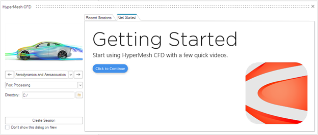
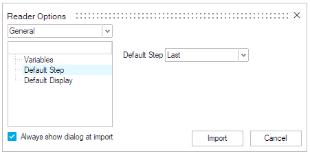
 The Derived Data Calculator opens.
 icon.
The default derived variable list is uploaded.
icon.
The default derived variable list is uploaded.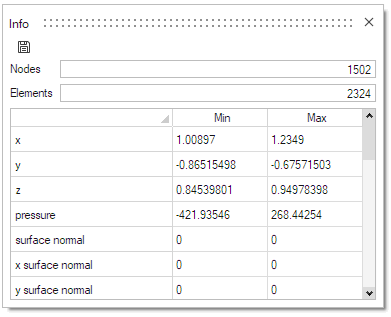 The Info micro-dialog opens.
 The Boundary Groups guide bar opens.
 button to open the Advanced
Selection dialog box.
button to open the Advanced
Selection dialog box.
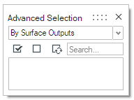 The Advanced Selection dialog Box opens.
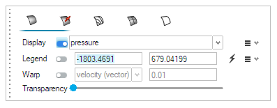

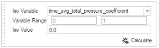 The Iso-Surfaces guide bar and Iso-Function guide panel open.
 The Box Clip guide bar opens.
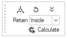 The Box Clip guide panel opens.
 The Scalar Clip guide bar opens.
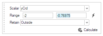 The Vehicle boundary group is highlighted, and the Scalar Clip guide panel opens..
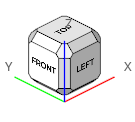
 The Views tool opens.
 button.
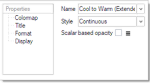 The Legend micro-dialog opens.
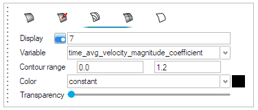
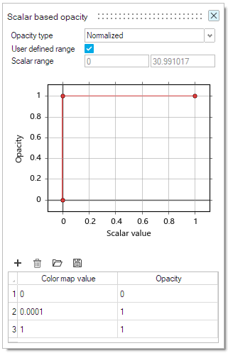 The Scalar Based Opacity dialog opens.
 The Surface Streamlines guide bar opens.
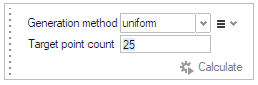
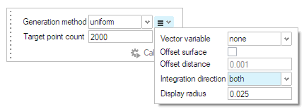 The Generation Method micro-dialog opens.
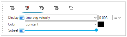 The Display Properties micro-dialog – Vector Display tab opens.
 The Legend Manager micro-dialog opens.
 The Slice Planes guide bar opens.
 The Slice Plane micro-dialog opens.
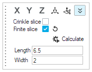
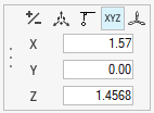 The Vector tool opens.
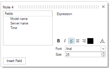

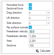
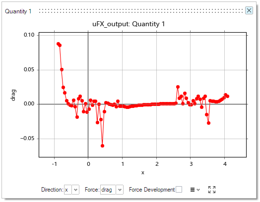 Note: This step uses significant computer resources and may take a few minutes to complete, depending on the machine.
 The Vortex Core guide bar opens.