From the horizontal toolbar, click File > Open > Solver Deck.
The File Browser opens.
From the File Browser, change the file type to STL
(*.stl).
Navigate to the provided tutorial directory where all the tutorial files are
stored, select the AhmedBody.stl
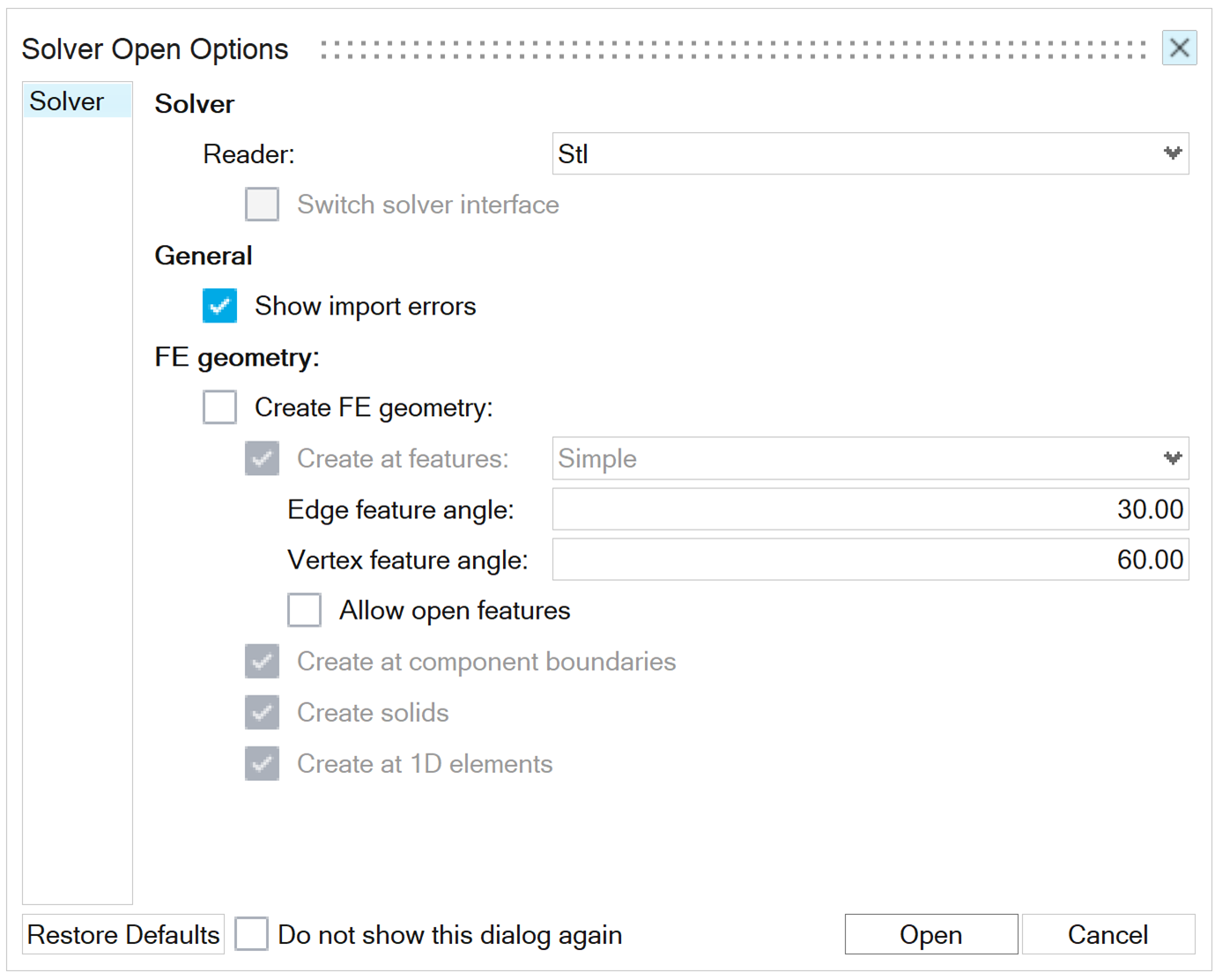
file and click Open. The Solver Open
Options dialog opens.
Figure 2.
Keep the default options and click Open.
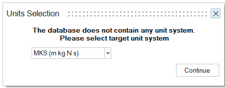
From the Units Selection dialog, select MKS
(m kg N s) and click Continue.
Figure 3.
From the horizontal toolbar, click File > Save As. The Save Session dialog opens. Navigate to
the tutorial root folder and for File Name enter
Model.hmcfd and click on Save
button.
From the Geometry ribbon, Home group, click on the Data
Transfer tool.
Figure 4.
In the guide bar, select Parts (selected by default) and
from the graphics area select the body part.
Activate the Clear existing Setup data option located
under the guide bar and click on Transfer.
Case Setup Environment Setup
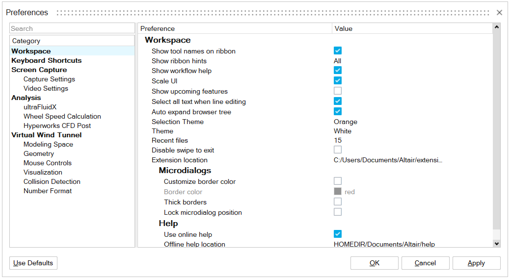
From the horizontal toolbar, click File > Preferences.
Figure 5. The Preferences dialog opens.
In the Preferences dialog, under Analysis, select
ultraFluidX and disable the
Compression preference.
Click Apply and then click OK to
close the Preference dialog.
Note: This step is being executed so the uFX solver deck
is written in .stl file format. In the later section of
the DOE study, for each simulation an .stl file that
corresponds to the shaped geometry will be created. The baseline model
.xml file will be the same for all simulations done
during the DOE.
From the horizontal toolbar, click View > Model Browser to activate the Model Browser. Repeat the
same step to activate the Property Editor. Both open on the
left side of the modeling window.
Note: The Model Browser and the Property Editor can also
be activated by pressing the F2 and F3 keys.
Define Wind Tunnel
From the Setup ribbon, click the Edit Tunnel tool.
Figure 6.
A tunnel is generated around the model.
In the Property Editor, under Inflow velocity set an
Inflow speed of 30 m/s.
In the Property Editor, under Tunnel
Properties, modify the dimensions of the wind tunnel:
For Length enter 16.7
m.
For Width enter 9.3
m.
For Height enter 6.7
m.
In the Property Editor, under Tunnel
Extents, enter -5.2 m for X
Min.
From the Model Browser, select the Wind
Tunnel and hide it with the H shortcut
key.
Define Mesh Controls
From the Setup ribbon, click on the Mesh
Controls tool.
Figure 7.
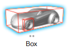
From the secondary tool set, click the Create Box Zone Around
Body tool.
Figure 8.
Select any location on the model’s body.
A new refinement box zone is created, and the Box
Zone micro-dialog appears.
From the Box Zone micro-dialog, click on the drop-down
arrows and set a value of 4 for
Level, 1.7 m for
Length, 0.6 m for
Width, 0.5 m for
Height and then press
Enter.
In the Property Editor, under Zone
Extents set a value of -0.25 m for
X Min and rename the created box by setting General > Name to Box_RL4.
From the Box Zone micro-dialog click on the
Plus button.
A second box refinement zone, which is one level coarser, is generated
around the initial one.
Repeat steps 4 to 6 using the following values:
Table 1.
Level
Name
Length
Width
Height
X Min
3
Box_RL3
2.4 m
0.8 m
0.5 m
-0.4 m
2
Box_RL2
3.1 m
0.95 m
0.7 m
-0.6 m
1
Box_RL1
5.2 m
1.1 m
0.85 m
-1.1 m
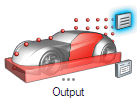
Define Output Controls
From the Setup ribbon, Output group, click on the General
Output tool. The ultraFluidX Output Controls dialog opens.
Figure 9.
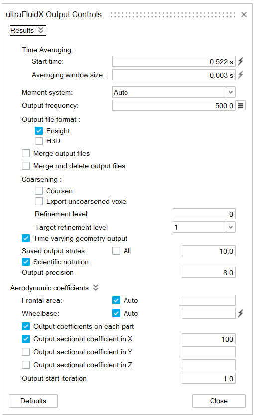
Figure 10.
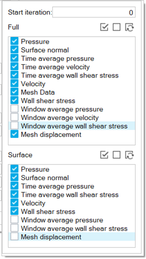
From the ultraFluidX Output Controls dialog:
Set the Output frequency value to
1.
Click on the hamburger menu of Results > Output frequency.
Figure 11.
The General Output Field Variables dialog
opens.
From the General Output Field Variables dialog:
Set the value of Start Iteration to
1616.
Note: From the
simulation parameters defined on the next section, iteration 1616 is
the last iteration of the uFX run. By selecting the latter as a
Start Iteration in combination with an
Output frequency of
1, only the last timestep of the
simulation will be exported for full & surface data.
For the Full data select
Pressure, Time average
pressure, Velocity,
Time average velocity and Surface
normal.
For the Surface data select
Pressure, Time average
pressure, Wall shear stress,
Time average wall shear stress.
From the Output file format enable
H3D and disable
Ensight.
Under Aerodynamic coefficients, enable sectional
coefficients in X, Y and Z and set a value of
100 sections for each of them. Leave
Output start iteration as
1.
Close the ultraFluidX Output Controls dialog.
Define Simulation Parameters
From the Setup ribbon, Run group,
click on the Run tool.
Figure 12.
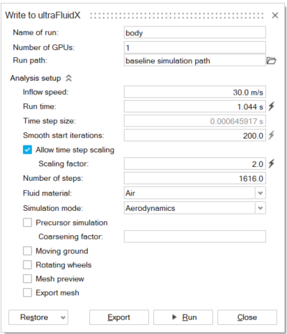
The Write to UltraFluidX dialog opens.Figure 13.
From the Write to UltraFluidX dialog:
Set the Name of run as
body, the Number of
GPUs as 1 and for Run
path set the path to the <working directory>/Study_Tutorial/baselineModel.
For the Scaling factor set a value of
2.
Uncheck the following options: Moving
ground, Rotating wheels,
Mesh preview.
The setting should be as follows:
Figure 14.
Click Export to export the solver deck in the simulation
directory.
From File > Save, save the .hmcfd session.
Post Automation File
An .img file has been created to utilize the Report
Generation utility of HyperMesh CFD. The file includes 2D plots of CL and CD
over time and the time averaged sectional CD. In the later section, 2D plots
will be generated for all the simulations completed in the DOE study, using this
.img file.
Morphing
Control Volumes
Switch to the Design Exploration environment.
From the Morphing ribbon, Setup
group, click the Volumes tool.
Figure 15.
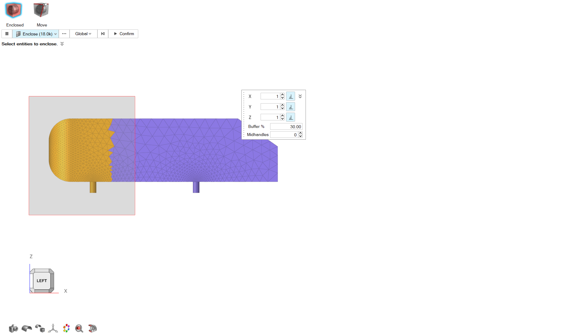
From the secondary tool set, click the Enclosed
tool.
Figure 16.
From the graphics area, select the elements at the front end of the body as
shown in the following figure.
Figure 17.
In the micro-dialog click on the arrow
to expand the drop-down menu. For Buffer %, set a value
of 30.
Click on Confirm to create the control volume.
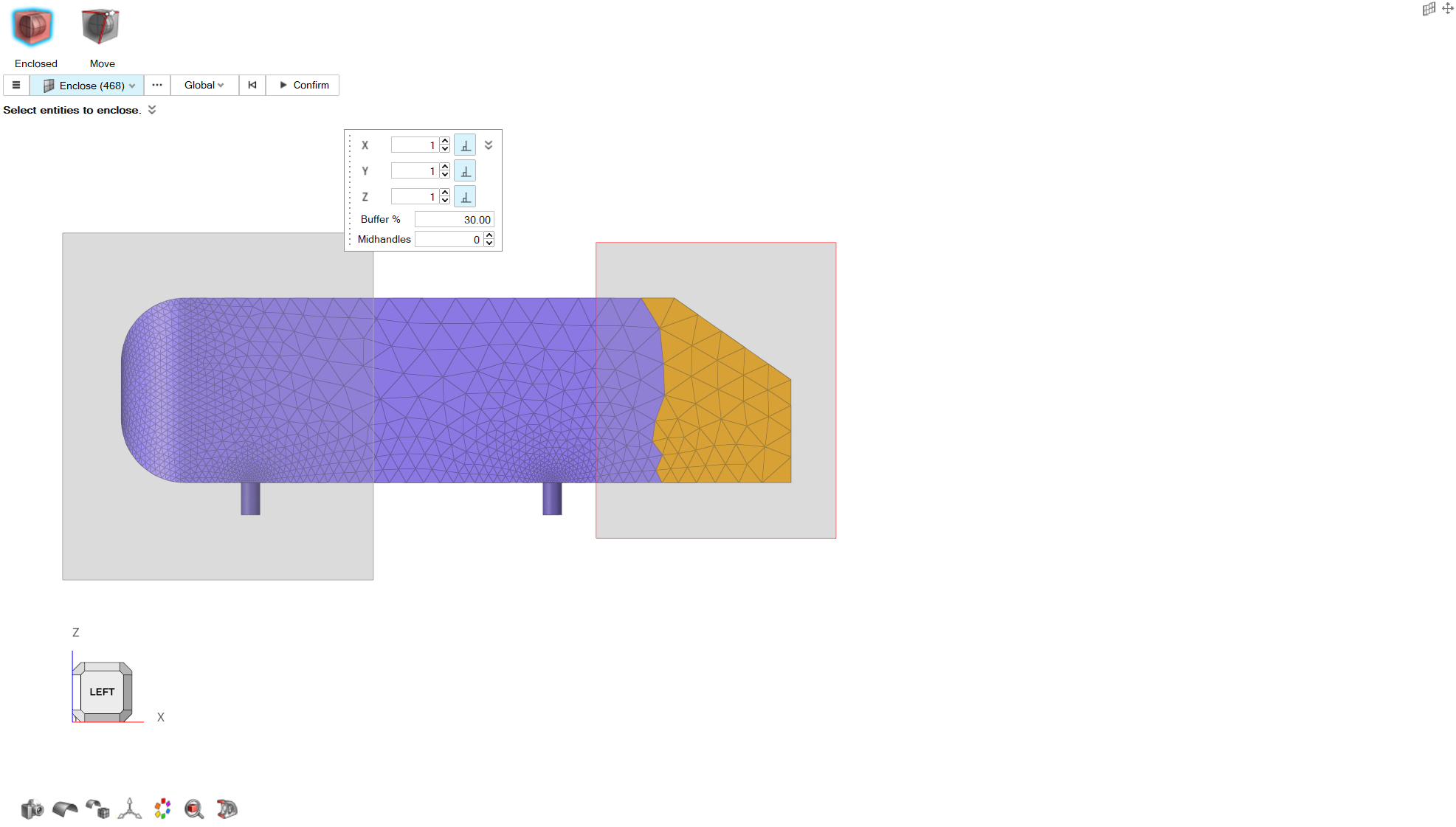
Repeat Steps 2 to 6 to create a second control volume as shown in the following
figure.
Figure 18.
Control Points
From the Morphing ribbon, Setup
group, click the Control Points tool.
Figure 19.
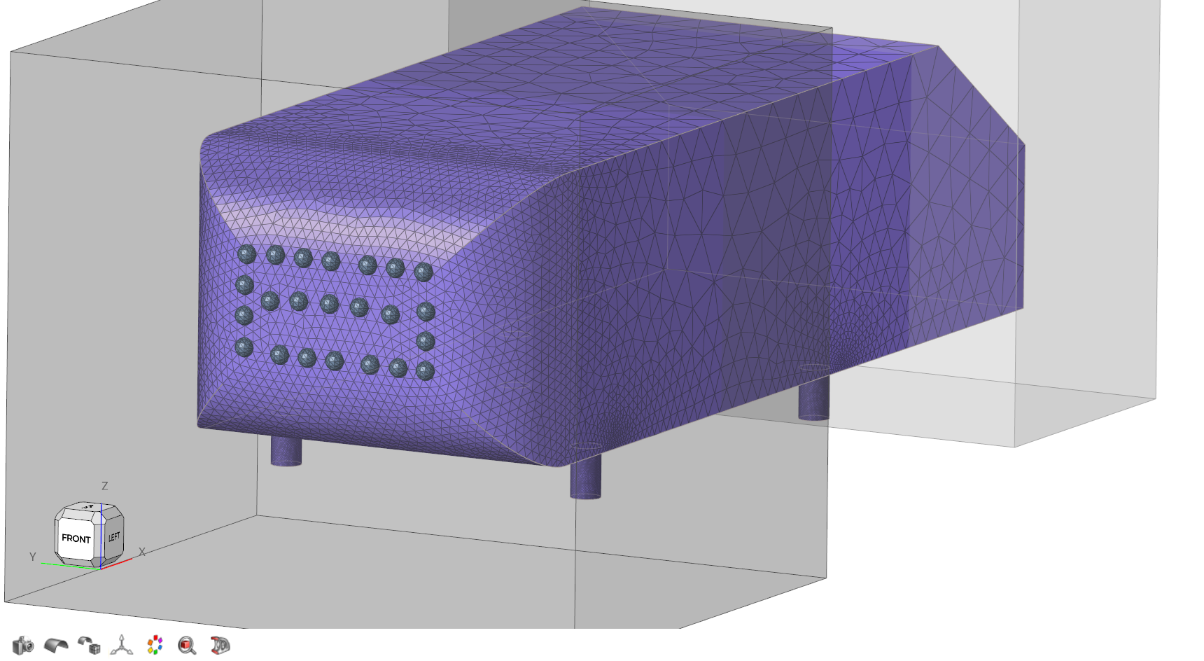
On the guidebar, select Seeds and create the following
control points on the front area of the model.
Figure 20.
Click Play on the guidebar to create the control points
set.
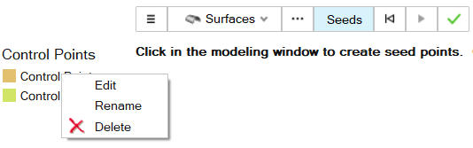
From the Control Points menu, right click on the newly
created control points and rename them to
shape2_front_active.
Figure 21.
Note: From the Seed Location
micro-dialog, use the Save icon to export control
point sets to .csv files. By using the
Folder icon, the user is able to import
previously saved or already existing control point sets from
.csv, .txt,
.dat files.
By clicking on the Seeds button on the guidebar, and
clicking within the graphics window, the Seed Locations
dialog opens.
From the Seed Locations dialog, select the created seed
and press the Delete button.
Click on the Folder icon from Seed
Location micro-dialog to import control points set from
shape2_fixed.csv file located in the
<working directory>/Study_Tutorial/Tutorial_StartFiles.
Click the Play button.
Rename the new set as
shape2_front_fixed from the Control Points
menu.
Morph
Shape 1
From the Morphing ribbon, Setup group click on the Morph tool.
Figure 22.
On the guidebar, select Parts and select the model from
the graphics area.
Note: Generally, it is important to select all the parts
we want to include in the geometry changes, to achieve better results in the
final geometry after the morph.
From the guidebar, click MorphVolumes and select the
control volume on the rear side of the model.
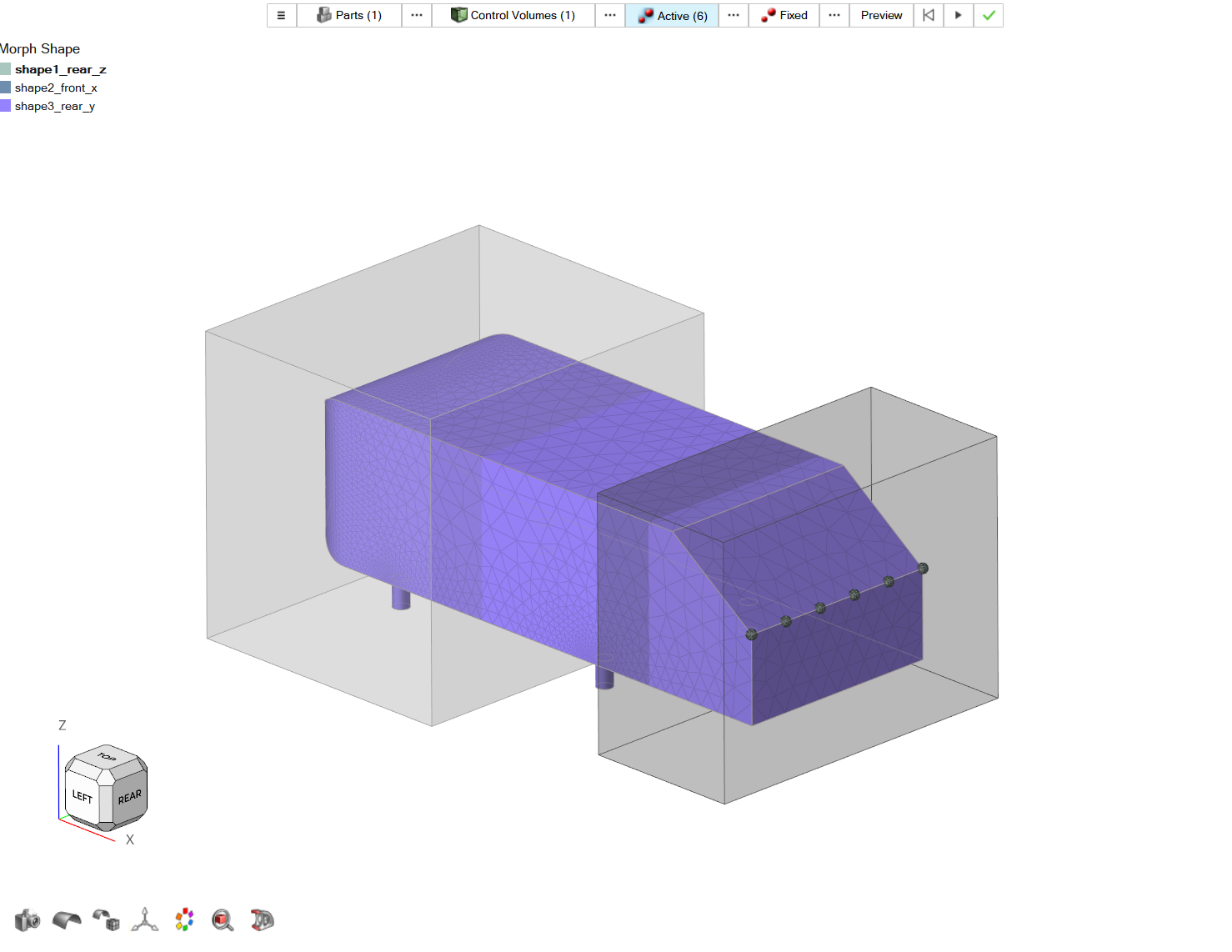
Click on Active on the guidebar and set the following
control points on the model.
Note: Attention is required while selecting the Active
control points of the morph, to keep the whole area of interest in the range
of the Impact Radius of these points (this will be clear later when we
visualize the resulting shape).
Figure 23.
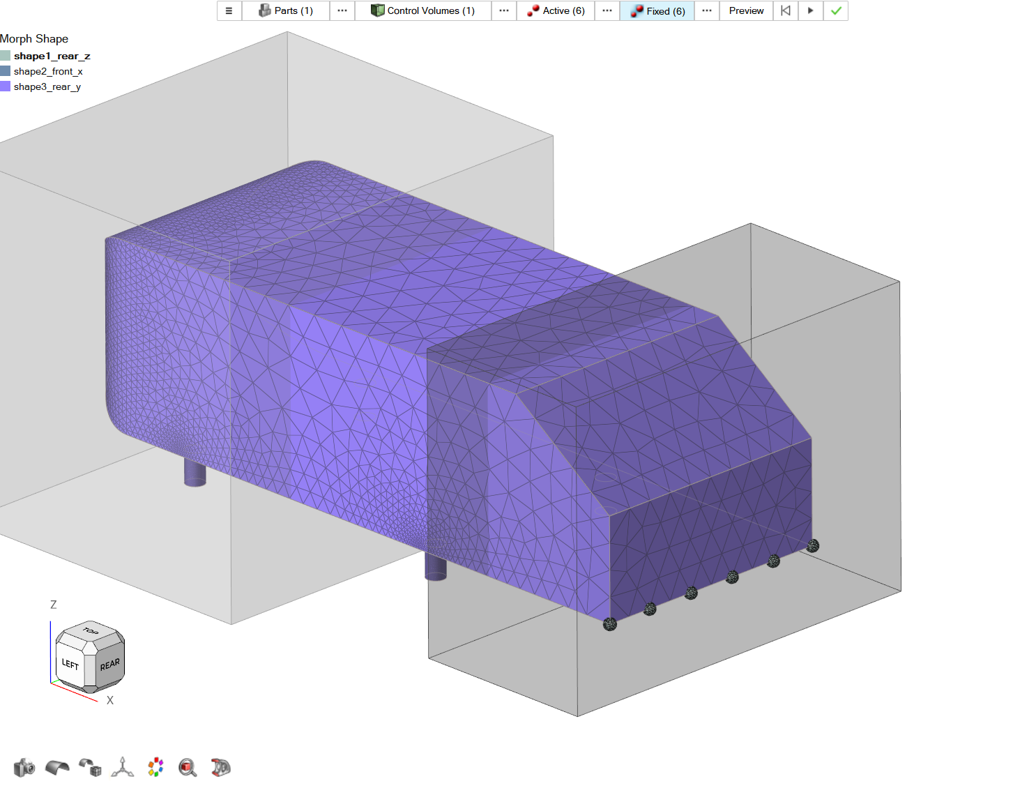
Click on Fixed from the guidebar and set the following control points on the
model.
Figure 24.
For the Translation Vector, set a Z
value of 0.05 m and let Impact
Radius as default with a value of 0.1
m.
Click on the Preview button and examine the displayed
morphed geometry.
If the shape describes the desired geometry sufficiently, click on the
Play button to create the shape.
From the Morph Shape menu, right click on the created
shape and rename it to shape1_rear_z.
Shape 2
From the tool’s guidebar, click on Parts and select the
model to create the next shape.
Click MorphVolumes from the guidebar and select the
control volume on the front side of the model.
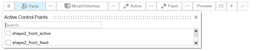
Click on Active and then click on the three dots button next to it on the
guidebar.
Figure 25.
The Active Control Points dialog
opens.
From the list select shape2_front_active and close the
dialog.
For the Translation Vector, set a X
value of -0.1 m and let Impact
Radius as default with a value of 0.1
m.
Click on Fixed and then click on the three
dots button
next to it on the guidebar.
The Fixed Control Points dialog opens.
From the list, select shape2_front_fixed and close the
window.
Click on the Preview button and examine the displayed
geometry.
Click on the Play button to create the shape and from
the Morph Shape menu, rename the newly created shape as
shape2_front_x.
Shape 3
Click on Parts in the guidebar and select the model to
create the next shape.
Click MorphVolumes from the guidebar and select the
control volume on the rear side of the model.
Click on Active and create the following control points
on the model.
Figure 26.
For the Translation Vector set a Y
value of 0.05 m and a value of
0.15 m for Impact
Radius.
Enable the Consider Symmetry option and set
Symmetry plane normal as (0, -1,
0).
Click on the Preview button and examine the displayed
geometry.
Click on the Play button to create the shape and from
the Morph Shape menu rename the newly created shape as
shape3_rear_y.
Shapes – Design Variables
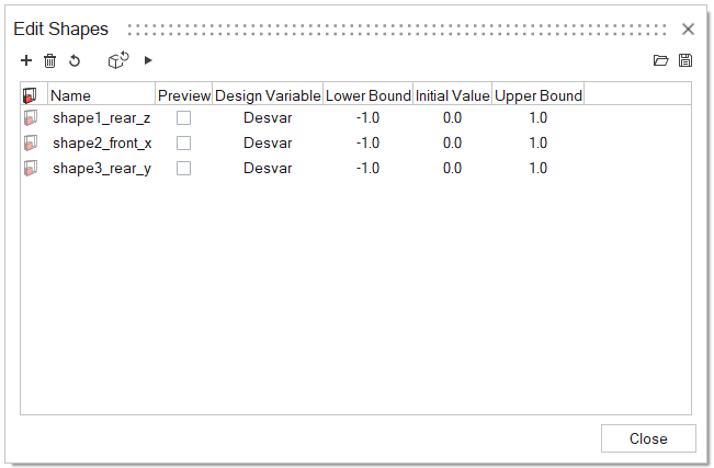
From the Review group click on the
Shapes tool.
Figure 27.
The Edit Shapes dialog opens.
Here you can select all three shapes and click on the Animate
Shapes button.
Figure 28.
Examine the created shapes by selecting them from the animation guidebar and
enabling Contour plot from the hamburger menu. Click on
the Display button on the guidebar to display the
currently applied factor or the current frame number.
Using the media arrow keys review different states of the morphed geometry for
factors 0.3, 0.6 and 0.8. Users can apply the shape with any factor between 0
and 1 by clicking on Shapes tool, selecting a shape of
interest, right click and select the option Apply by
Factor. This action will open a pop-up dialog where the user is
able to specify any desired factor for this shape preview.
Click on the green check arrow to exit the animation.
From the Edit Shapes dialog, under the Design
Variable column specify all the shapes as Desvar. Make sure the
following values are kept: Lower Bound =
-1, Initial value =
0, Upper Bound =
1.
Figure 29.
Click on Close.
Design of Experiment (DOE)
Launch HyperStudy
From the DOE group click on the DOE
Study tool.
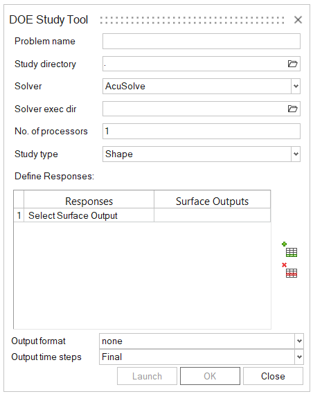
The DOE Study tool dialog opens.Figure 30. Figure 31.
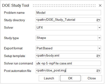
From the DOE Study tool dialog:
Set the Problem name as
Model.
Note: The
Problem Name and the
.hmcfd model name must be the
same.
To set the Study directory, click on the Folder
icon and navigate to the <working
directory>/Study_Tutorial folder and select the
DOE_Study_Tutorial directory.
Set the Solver to
UFX.
Set the Study type to
Shape.
Set the Export format to Part
Based.
To set the Setup template file, in this tutorial the
baseline model .xml file will be used. Click on the
Folder icon and navigate to the baseline model solver
deck location and select body.xml file.
Note: To run ultraFluidX simulations, the installation
must include hwcfdsolvers.
(For Linux users) Set the Solver run command “<HMDesktop
Installation folder>/altair/hwcfdsolvers/scripts/ufx" -np 2 -inpFile
body.xml..
To set the Post automation file click on the
Folder icon and navigate to <working
directory>/Study_Tutorial. Select the
doe_post.img file.
Figure 32.
Click Launch to launch the HyperStudy client.
Setup – Nominal Model
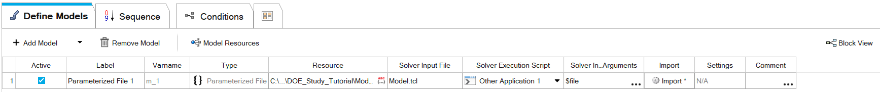
From the Study Explorer on the left-hand side under Setup > Definition, click on Define Models. Here you can find
general details about the model.
Figure 33.
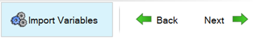
Click on Import Variables to import the shape Design
Variables created in the Design Exploration environment of HyperMesh CFD. Click
on the Next button.
Figure 34.
Review the Input Variables and click on the Next
button.
From Study Directory, right click on
Ufx_Hst file. Select Show In > Explorer.
(For Linux users) Open Ufx_Hst file in the text
editor.
Update the hmbatch script’s path to
“$HW_ROOT/scripts/hmbatch”.
Before the execution command of hwcfdReport script, add the following
line of code: cp “<working directory>/Study_Tutorial/doe_post.img”.
Update the hwcfdReport script’s path to
"$HW_ROOT\hwx\plugins\hwd\profiles\HyperworksCfd\hwcfdReport".
Make sure the input to hwcfdReport script is specified as:
--img doe_post.img
Before the hwcfdReport call command, make sure to add the following
lines of
code:
while [ ! -e "uFX_summary.txt" ]
do
# Check if termination text is present in uFX log
if grep -1 "terminating" "uFX_log_*" then OR if grep -q -e "terminating" -e "Error:" "uFX_log_*"; then
break
fi
sleep 10
done
(For Linux Users) Click on Run Definition button. The
model files and settings files are written, then the baseline simulation should
begin. When all tasks are completed, click on the Next
button to continue.
Windows users, where ultraFluidX cannot work, will continue with the Test
Models step (Step 8) and then will copy paste the simulation files in the
corresponding folder under the study directory. Once this is done the user will
be able to continue the setup.
(For Windows users) Extract and copy ultraFluidX
simulation data in the DOE subdirectory.
In the Test Models tab, click on the
Write button. The model files and settings
files are written.
From the Study Directory, click on the approaches
folder, select Show In > Explorer.
Extract and then Copy the baseline simulation files located at
<working directory>/Study_Tutorial
/hst_files_for_windows_users/setup_1-def/m_1.
Navigate to approaches/setup_1-def/run__0001/m_1/
folder and Paste the copied files.
Return to HyperStudy environment. In the Test
Models tab, click on the Extract
button. Then click on the Next button to
continue.
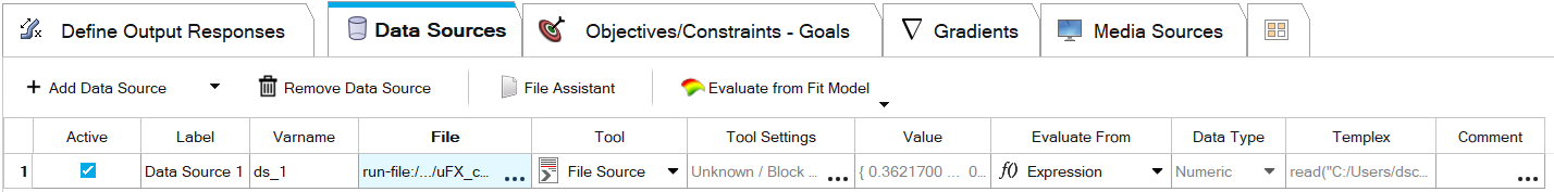
Click on the Data Sources tab. Then, click on the
Add Data Source button.
Figure 35.
A new variable line appears.
From the File column click on the three dots.
The Data Source Builder dialog opens.
From the File option, click on the Folder
icon and navigate to the
uFX_coefficients_Avg.txt file under
approaches\setup_1-def\run__00001\m_1\uFX_coefficientsData
folder. Select and click Open.
Figure 36.
From the Component drop down menu, select
Column 2, which describes the CX coefficient.
Click OK.
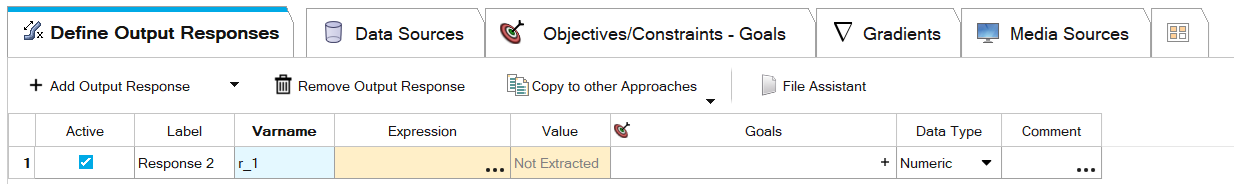
Click on the Define Output Responses tab and then click on
Add Output Response button.
A new variable line appears.Figure 37.
Under the Expression column click on the three
dots button.
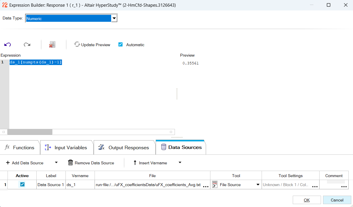
The Expression builder dialog opens.Figure 38.
Click on the Data Sources tab.
From the Data Sources tab, click on the Insert
Varname arrow to expand the drop-down menu. From the list,
select the Last Element option and then click on the
Insert Varname button.
The resulting value is displayed in the Preview
area.
Click OK.
Design of Experiment Study
Click on the Next button. Two options appear, select
Add.
In the window that pops up, under Select Type select
DOE. In the Definition From
drop down menu select Setup. Click
OK to continue.
Figure 39.
In the Study Explorer under DOE 1,
repeat the model definition as previously done for Setup on Steps 2 to 3.
The Test Models step can be skipped. The DOE is Setup
based, and the nominal uFX simulation is already completed during the Setup
Definition of the study. Input Variables and Output Response definitions are the
same as specified earlier, during the Setup Definition.
Click on the Next button twice.
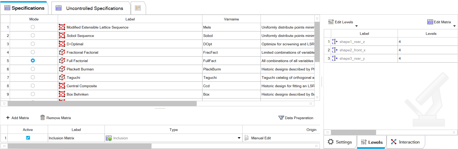
Under the Specifications tab, click on Show
more and select the Full Factorial DOE
Method.
On the right-hand side of the HyperStudy window, select the
Levels tab to specify levels for Input
Variables. Specify a Level value of
4.
Figure 40.
Click on Apply and then click on the
Next button.
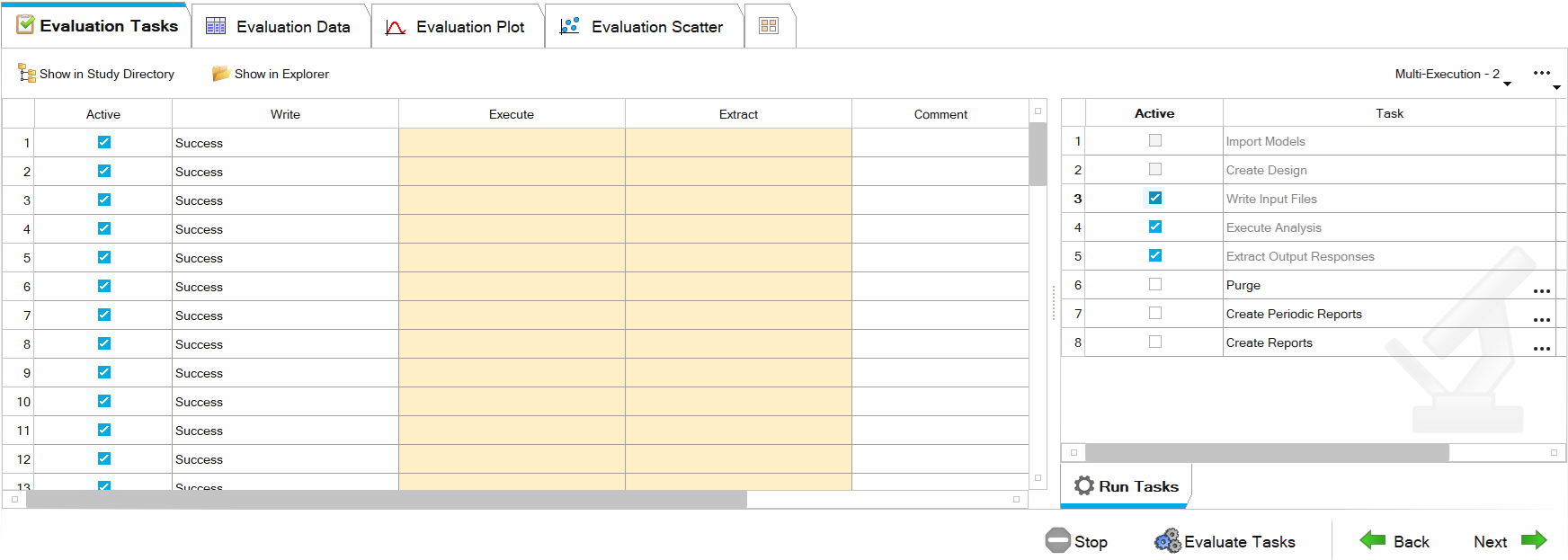
At the Evaluate step, on the Run
Tasks selection, enable only the Write Input
Files option and click the Evaluate Tasks
button. This will create directories for all the runs of the DOE under the
<working directory>/Study_Tutorial/DOE_Study_Tutorial/approaches/doe_1
subfolder. Also, the setting files for each run will be created.
Figure 41.
If every run’s Write column is tagged as Success, on the
Run Tasks selection enable Execute
Analysis and Extract Output Responses
options.
Note: For this tutorial, the desired result files from the
DOE study are provided. Running the complete analysis is a time-heavy task
that might take several hours for the user to complete (depending on the
available resources). It is suggested that the user completes only a small
amount of simulations (1 to 4) to be able to explore the Post-Processing
capabilities.
(For Linux Users) In the Evaluation Tasks tab, activate cases 1 to 4. Click on
the Evaluate Tasks button to run the DOE study.
Note: (For Windows users) Copy and paste the simulation
files into the corresponding folder under the study directory.
(For Windows users) Extract and copy ultraFluidX simulation data in the DOE
subdirectory.
From the Study Directory, right click on the
approaches folder, select Show In > Explorer.
Extract and then Copy the
DOE simulation file folders from <working
directory>/Study_Tutorial
/hst_files_for_windows_users/doe_1/.
Navigate to the <working
directory>/Study_Tutorial/DOE_Study_Tutorial/approaches/doe_1/
folder and Paste the copied files.
Return to HyperStudy environment. In the Run Tasks
tab, enable only the Extract Output Responses
task and click the Evaluate Tasks button.
When all tasks have been completed and every step in the Study
Explorer is highlighted as green, continue to the Post-Processing
step by clicking on the Next button.
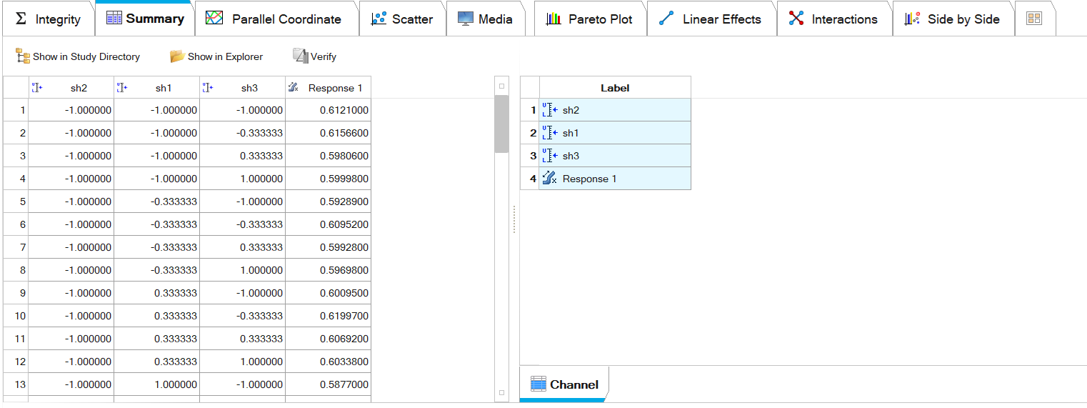
Under the Summary tab, a table with the Response Output
values per Input Variables pair is displayed. This can be used to further
organize your study on the model if needed. The enumeration matches the
Evaluation Tasks order.
Figure 42.
Note: More options for visualization on the DOE results,
based on the response outputs and input variables, can be found in this
step. Linear Effects, Interactions and Pareto Plot are some useful plots to
use to see how each shape’s input variable value interacts with the response
output, CX, behavior.
Save the current study. Close the HyperStudy window and return to the HyperMesh
CFD session that is already open.
PhysicsAI
Create a PhysicsAI Project
From the ribbon selection toolbar (horizontal toolbar), select
PhysicsAI.
From the PhysicsAI ribbon, click on the Create
Project tool.
Figure 43.
The Create Project dialog opens.
From the Create Project dialog
For Project Name, enter
Ahmed_Body_PAI.
For Location, click on Pick
Location and select a save location for the
project.
Click OK.
Decimate Utility (Optional)
In case the DOE was not conducted or fully completed, the
decimated .h3d files are already provided within the working directory (<working directory>/Study_Tutorial/decimated_surfaceData_h3ds.zip). If the provided
.h3d files are used, this section can be skipped. If so,
proceed directly to the Create Datasets
section of the tutorial.
From the PhysicsAI ribbon, click on the
Decimate tool.
Figure 44. Figure 45.
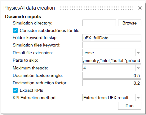
The PhysicsAI Data Creation dialog
opens.
For Simulation Directory, click on the
Browse button.
The Simulation Directory dialog opens.
Navigate to the
Study_Tutorial/DOE_Study_Tutorial/approaches/doe_1
folder and click Select Folder. This folder contains all
the runs that were executed during the DOE.
Enable the Consider Subdirectories for File
checkbox.
For Folder Keyword to Skip, enter
uFX_fullData and uFX_meshData.
These keywords will be used to skip folders during search.
For Simulation Files Keyword, leave it blank.
For Result File Extension, click on the arrow to expand
the drop-down menu, and select .h3d.
For Parts to Skip, ensure it is blank.
Note: The parts defined in the Parts to
Skip tab are completely removed during decimation and they
are not included in the resulting decimated result file.
For Maximum Threads, leave it as default.
For Decimation Feature Angle, enter
1.
For Decimate Reduction, enter
0.2.
Enable the Extract KPIs checkbox.
For KPI Extraction Method, click on the arrow to expand
the drop-down menu, and select Extract from UFX
result.
Click on Run.
After the decimate tool has finished, navigate to the <working directory>/Study_Tutorial/DOE_Study_Tutorial/Approaches/doe_1 folder
and notice that a new folder under the name h3ds has been
created. This folder contains both the decimated result files and the
.json files needed for KPI predictions.
Create Datasets
Training and Testing Datasets
From the PhysicsAI ribbon, click on the Create
Dataset tool.
Figure 46.
Figure 47.
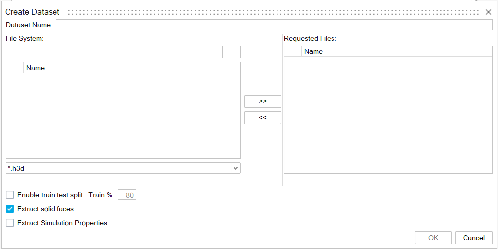
The Create Dataset dialog opens.
For Dataset Name, enter
Ahmed_Body.
For File System, click on the three dots button.
The Select Folder dialog opens.
From the Select Folder dialog, navigate to the folder
where the decimated .h3d files are stored and click
Select Folder.
The table under File System should now be populated with
all the decimated .h3d files.
Note: Under the File System table,
the desired file type can be specified for file selection. By default, it is
set as *.h3d.
Note: In this case, the result files contained field
information, such as pressure and wall shear stress fields. However, in case
vector data are the only output (such as Key Performance Index studies), the
geometry information can be supplied using mesh files, such as
.fem files.
Select all .h3d files and click on the transfer button to
transfer them to the Requested Files table.
Enable the Enable Train Test Split option and make sure
the Train % is set to 80.
The Enable Train Test Split option will automatically
split the selected files into two datasets, one used for training and one used
for testing. By default, the train percentage is set to 80%, which means that
80% of the specified h3d files will be put in the training dataset, while the
rest will be put in the testing dataset.
Enable the Extract Solid Faces option.
Disable the Extract Simulation Properties option.
Click OK.
After the extraction of the training dataset is done, the
Datasets dialog opens.
Figure 48.
Note: Notice that due to the use of the Enable
Train Test Split option, two datasets are created, one for
training and one for testing.
Click Close.
PhysicsAI for KPI Predictions
In this section a PhysicsAI model will be trained with the
SER method to predict drag coefficient values.
Train the Machine Learning Model
From the PhysicsAI ribbon click on the Train ML Model
tool.
Figure 49. Figure 50.
The Train Model dialog opens.
From the Train Model dialog:
For Model Name, enter
Ahmed_Body_SER.
For Training Data, select
Ahmed_Body_train.
Under Methods, select SER.
On the right-hand side of the Train Model dialog,
the SER method hyperparameters are shown.
Note: PhysicsAI offers three methods for training, the
Graphic Neural Simulator (GCNS), the Transformer Neural Simulator (TNS) and
the Shape Encoding Regressor (SER). The GCNS and TNS methods can be used for
field variable predictions, while SER is solely used for KPI predictions.
For more information on these methods refer to the PhysicsAI help
page.
Note: Once the SER method has been selected, the Inputs
and Outputs > Contours tabs become unavailable for modification.
Under Outputs > Vector, select Cx.
Specify the hyperparameters as shown in the table below:
Table 2. SER Hyperparameters
Hyperparameters
Values
K-fold Builds
10
K-fold Test Fraction
0.1
PCA Input
Enabled
PCA output
Disabled
Note: You can click on the hyperparameter names to read
their description.
Click Train.
Note: Training may take some time, depending on the
available resources. An already trained SER model is also provided in the
<working directory>/Study_Tutorial/PhysicsAI_Trained_Models folder. This
model can be used to continue the tutorial by importing it through the
Import Model button in the Model
Training dialog.
Figure 51.
The Model Training dialog opens.
After training is completed, the Status will change to
Done.
Click on Set Active Model and then click on
Close to exit the Model Training
dialog.
Test the Machine Learning Model
Using the Model Testing tool, predictions on models, whose
CFD results are available, can be generated. The Model Testing tool automatically
calculates metrics to assess the Machine Learning model’s performance.
From the PhysicsAI ribbon click on the Test ML Model
tool.
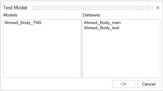
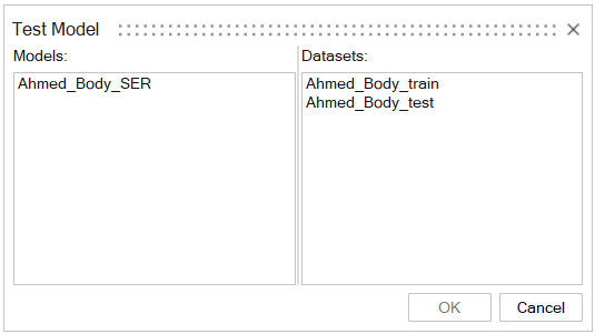
The Test Model dialog opens.Figure 52. Figure 53.
From the Test Model dialog, under
Models, select Ahmed_Body_SER.
Under Datasets select
Ahmed_Body_test.
Click OK.
Note: In this case, due to the small size of the models,
testing takes very little time to complete. Notice that for larger models it
may take longer, depending on the models’ sizes.
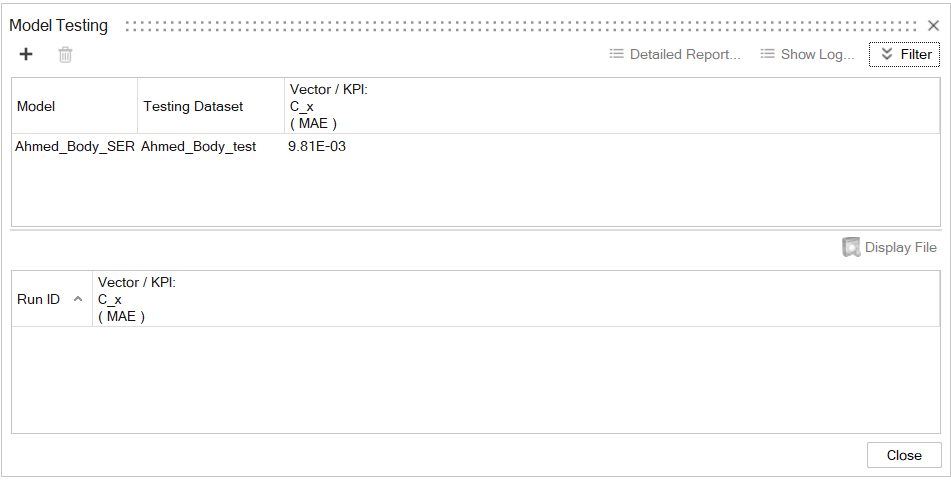
After testing is completed, the Model Testing dialog
opens.
Figure 54.
In the Model Testing dialog, the Mean Absolute Errors
(MAE) for the specified Vector Outputs over all test models are displayed.
Click on the Ahmed_Body_SER model. The Run IDs along with
their corresponding MAEs are displayed.
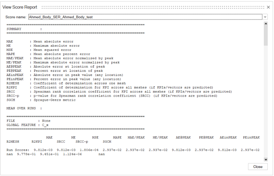
Click on Detailed Report to open the View
Score Report dialog.
Figure 55.
Click Close to exit the View Score
Report dialog.
Note: From the Model Testing dialog,
select an individual Run ID and click Display File.
The PhysicsAI Plot windows opens, displaying the true
and predicted Cx values for the selected model in a plot.
Click Close to exit the Model
Testing dialog.
Predict Using the Machine Learning Model
Using the Predict tool, you can
generate predictions for new designs.
Morphing
From the ribbon selection toolbar (horizontal toolbar), select
Morphing.
From the Setup group, click on the
Volumes tool.
From the secondary tool set, click on the Enclosed
tool.
From the graphics area, select the elements at the front end of the body as
shown in the following figure,
In the micro-dialog click on the arrow to expand the drop-down menu. For Buffer
% set a value of 30.
Figure 56.
Click Confirm to create the control volume.
From the Morphing ribbon, Setup
group, click on the Control Points tool.
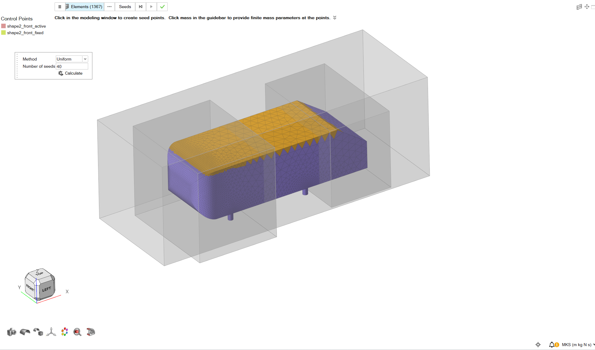
On the guidebar set the selector to Elements.
From the graphics window, select the following elements.
Figure 57.
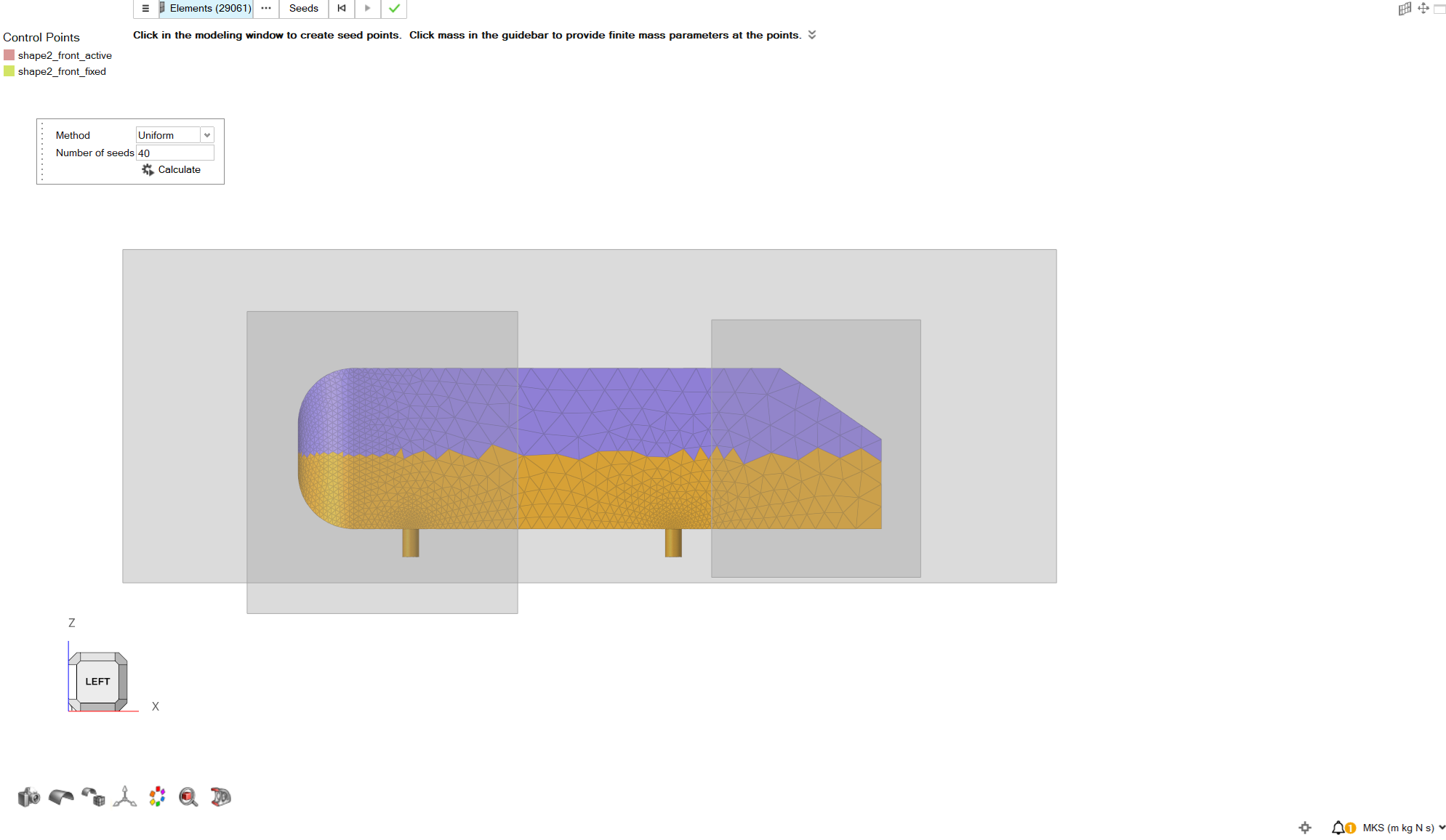
In the micro-dialog, select Uniform option for
Method, and a target Number of
seeds of 40.
Click on the Calculate button to create the control
points set.
Close the Seed Location dialog.
From the Control Points menu, right-click on the newly
created control points and rename them to
Predict_Active.
Repeat Steps 7-12 for the elements shown in the following image.
Figure 58.
From the Control Points menu, right click on the newly
created control points and rename them to
Predict_Fixed.
Click on the green check arrow to exit the tool.
From the Morphing ribbon, Setup group
click on the Morph tool.
On the guidebar, select Parts and select the model from
the graphics area.
On the guidebar, click MorphVolumes and select the
control volume created in Step 6.
Click on Active on the guidebar. Then click on the 3-dot
button next to it in the guidebar. From the
Active Control Points dialog, select
Predict_Active set. Close the Active Control
Points dialog.
Click on Fixed on the guidebar. Then click on the 3-dot
button next to it in the guidebar. From the
Fixed Control Points dialog, select
Predict_Fixed set. Close the Fixed Control
Points dialog.
For the Translation Vector set a Z
value of -0.05 m in the and let
Impact Radius as default with a value of
0.1 m.
Click on the Preview button and examine the displayed
morphed geometry.
Click on the Play button to create the shape.
From the Morph Shape menu right click on the created shape
and Rename it to
PredictDesign.
Click on the green check arrow to exit the tool.
From the Review group click on the
Shapes tool.
Select PredictDesign shape and right click on it, then
click on Apply by Factor button. A micro-dialog opens.
Set a value of 1 and click on
Apply.
Close the Edit Shapes dialog.
Prediction
Once the new morphed design has been created and applied, from the PhysicsAI
ribbon click on the Predict tool.
Figure 59.
Note: If a “No Active PhysicsAI Model” error gets
displayed, go to Model Training, select the
Ahmed_Body_SER model, then click Set
Active Model.
After a prediction is generated, the PhysicsAI Plot
windows opens, displaying the predicted Cx value for the morphed
model.
PhysicsAI for Field Variable Predictions
In this section a PhysicsAI model with the TNS method will
be trained to predict time average pressure and time average wall shear stress
fields.
Note: For GCNS and TNS, it is advised to train
PhysicsAI models using a GPU, because it is significantly faster than training on a
CPU. To use a GPU for training, please refer to PhysicsAI
help.
Train the Machine Learning Model
From the PhysicsAI ribbon, click on the Train ML Model
tool.
Figure 60. Figure 61.
The Train Model dialog opens.
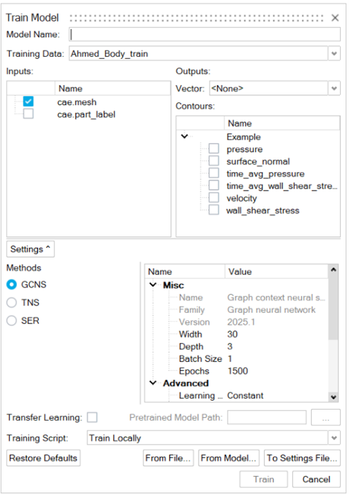
From the Train Model dialog
For Model Name, enter
Ahmed_Body_TNS.
For Training Data, select
Ahmed_Body_train.
Under Methods, select TNS.
On the right-hand side of the Train Model dialog,
the TNS method hyperparameters are shown.
Under Inputs, select
cae.mesh and make sure that the
cae.part_label is not selected.
Note: Using the cae.mesh option as
input means that the spatial coordinates are used as a predictor of
behavior. This option is selected by default, and it is recommended to
always keep it on.
Note: The cae.part_label allows for
part labels to be used as predictors of behavior. It is useful in the case
of large assemblies, where part names remain unchanged. However, it is
suggested to turn it off if there are changes in part naming. By default,
cae.part_label is not selected.
Under Outputs > Contours, select time_avg_pressure and
time_avg_wall_shear_stress.
Specify the hyperparameters as shown in the table below.
Table 3. TNS Hyperparameters
Hyperparameters
Values
Width
64
Depth
4
Sections
32
Attention Heads
4
Node Subsampling Fraction
0.5
Batch Size
1
Epochs
600
Learning Rate
Cosine Decay
Initial Value
1e-3
Decay Fraction
1e-3
Early Stopping
Enabled
Patience
100
Mesh Alignment
None
Validation Fraction
0.15
Note: You can click on the hyperparameter names to read
their description.
Click Train. The Model Training dialog opens.
Note: Training may take some time, depending on the
available resources. An already trained TNS model is also provided in the
<working directory>/Study_Tutorial/PhysicsAI_Trained_Models folder. This
model can be used to continue the tutorial by importing it through the
Import Model button in the Model
Training dialog.
Figure 62.
Note: Once the Status changes to
Running, click on Show Log to inspect the training
log file or click on Loss Curve to monitor the
progression of the training and validation losses.
After training is completed, the Status will change to
Done.
Click on Set Active Model and then click on
Close to exit the Model Training
dialog.
Test the Machine Learning Model
Using the Model Testing tool, you can generate predictions
on models, whose CFD results are available, and automatically calculate metrics to
assess the Machine Learning model’s performance.
From the PhysicsAI ribbon click on the Test ML Model
tool.
Figure 63.
The Test Model dialog opens.Figure 64.
From the Test Model dialog, under
Models select Ahmed_Body_TNS.
Under Datasets select
Ahmed_Body_test.
Click OK.
Note: In this case, due to the small size of the models,
testing takes about a minute to complete. Notice that for larger models it
may take longer, depending on the models’ sizes.
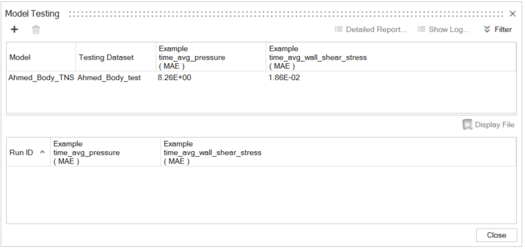
After testing is completed, the Model Testing dialog
opens.
Figure 65.
In the Model Testing dialog, the Mean Absolute Errors
(MAE) for the specified Outputs over all test models are displayed.
Click on the Ahmed_Body_TNS model. The Run IDs along with
their corresponding MAEs are displayed.
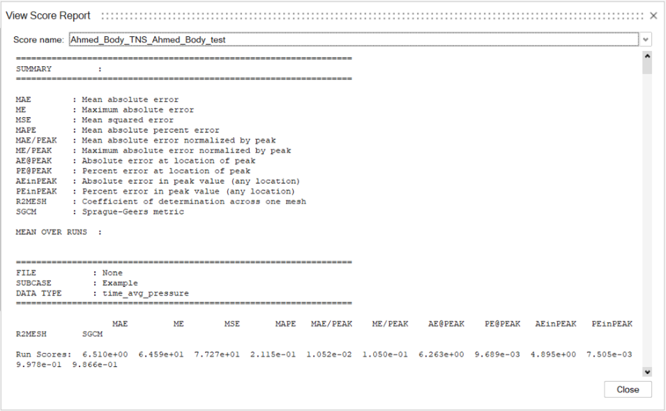
Click on Detailed Report to open the View
Score Report dialog.
Figure 66.
Click Close to exit the View Score
Report dialog.
Note: From the Model Testing dialog,
select an individual Run ID and click Display File.
HyperMesh CFD automatically switches to the Post-Processing environment and
loads the prediction and true results for the selected Run ID.
Click Close to exit the Model
Testing dialog.
Predict Using the Machine Learning Model
Using the Predict tool, you can generate predictions for
new model designs.
Morphing
From the ribbon selection toolbar (horizontal toolbar), select
Morphing.
From the Setup group, click on the
Volumes tool.
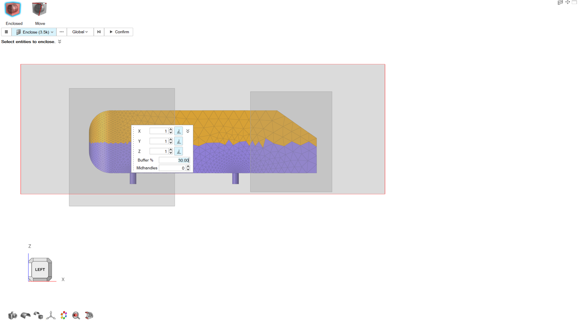
From the secondary tool set, click on the Enclosed
tool.
From the graphics area, select the elements at the front end of the body as
shown in the following figure.
In the micro-dialog click on the arrow to expand the drop-down menu. For Buffer
% set a value of 30.
Figure 67.
Click Confirm to create the control volume.
From the Morphing ribbon, Setup
group, click the Control Points tool.
On the guidebar set the selector to Elements.
From the graphics window select the following elements.
Figure 68.
In the micro-dialog select Uniform option for
Method, and a target Number of
seeds of 40.
Click on the Calculate button to create the control
points set.
Close the Seed Location dialog.
From the Control Points menu, right click on the newly
created control points and rename them to
Predict_Active.
Repeat Steps 7 to 12 for the elements shown in the following image.
Figure 69.
From the Control Points menu, right click on the newly
created control points and rename them to
Predict_Fixed.
From the Morphing ribbon, Setup group
click on the Morph tool.
On the guidebar select Parts and select the model from
the graphics area.
On the guidebar click MorphVolumes and select the
control volume created on Step 6.
Click on Active on the guidebar. Then click on the 3-dot
button next to it in the guidebar. From the
Active Control Points dialog, select
Predict_Active set. Close the Active Control
Points dialog.
Click on Fixed on the guidebar. Then click on the 3-dot
button next to it in the guidebar. From the
Fixed Control Points dialog select
Predict_Fixed set. Close the Fixed Control
Points dialog.
For the Translation Vector set a Z
value of -0.05 m in the and let
Impact Radius as default with a value of
0.1 m.
Click on the Preview button and examine the displayed
morphed geometry.
Click on the Play button to create the shape.
From the Morph Shape menu right click on the created shape
and rename it to PredictDesign.
From the Review group click on the
Shapes tool.
Select PredictDesign shape and right click on it, then
click on Apply by Factor button. A micro-dialog opens up.
Set a value of 1 and click on
Apply.
Close the Edit Shapes window.
Prediction
Once the new morphed design has been created and applied, from the PhysicsAI
ribbon click on the Predict tool.
Figure 70.
Note: If a “No Active PhysicsAI Model” error gets
displayed, go to Model Training, select the
Ahmed_Body_TNS model and click Set
Active Model.
Note: The predicted .h3d file will be
saved in the directory specified in the Create Session
dialog.
After a prediction is generated for the morphed model, the environment will
automatically switch to Post-Processing, where the predicted results will be
available for visualization.
In the Post-Processing environment of HyperMesh CFD the drag coefficient of
the design can also be calculated.
From the Post-Processing environment,
Measures group, click on the Engineering
Quantities tool.
Figure 71.
From the guidebar, select Force and set the selector to Boundary Groups. Then,
from the graphics window, select the body boundary group.
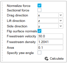
A micro-dialog with optional calculation parameters comes
up.
From the micro-dialog, enable the checkboxes for
Normalize force, Flip surface
normals, and set the Freestream velocity
as 30 m/s, the Freestream density
as 1.2041 kg/m3, and the Area as
0.1 m2.

 A tunnel is generated around the model.
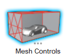
 The General Output Field Variables dialog opens.
 The Write to UltraFluidX dialog opens.
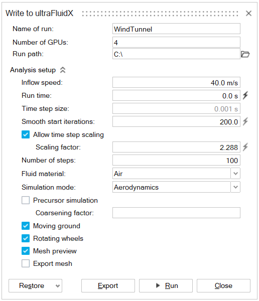

 to expand the drop-down menu. For Buffer %, set a value
of 30.
to expand the drop-down menu. For Buffer %, set a value
of 30.
 Note: From the Seed Location micro-dialog, use the Save icon to export control point sets to .csv files. By using the Folder icon, the user is able to import previously saved or already existing control point sets from .csv, .txt, .dat files.
 .
.
 The Active Control Points dialog opens.
 next to it on the guidebar.
The Fixed Control Points dialog opens.
next to it on the guidebar.
The Fixed Control Points dialog opens.
 The Edit Shapes dialog opens.
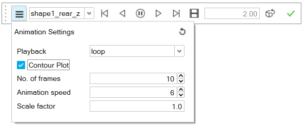
 A new variable line appears.
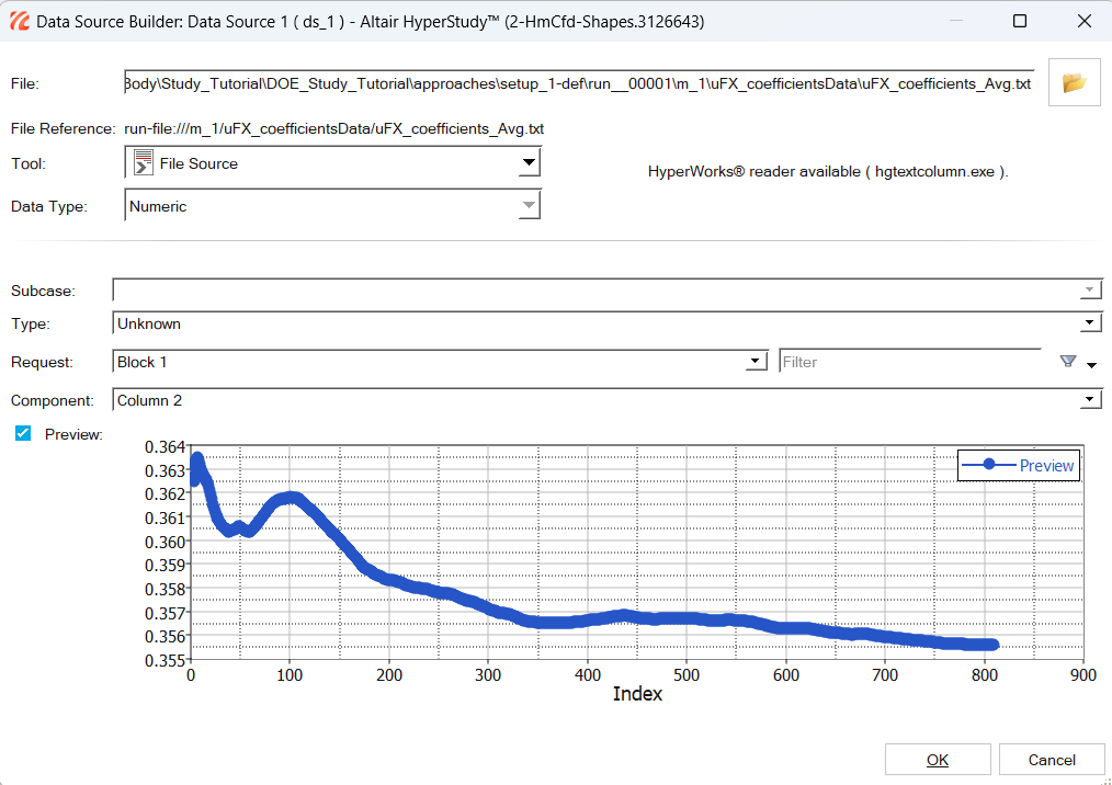

 Note: More options for visualization on the DOE results, based on the response outputs and input variables, can be found in this step. Linear Effects, Interactions and Pareto Plot are some useful plots to use to see how each shape’s input variable value interacts with the response output, CX, behavior.
 The Create Project dialog opens.
 The PhysicsAI Data Creation dialog opens.
 The Create Dataset dialog opens.
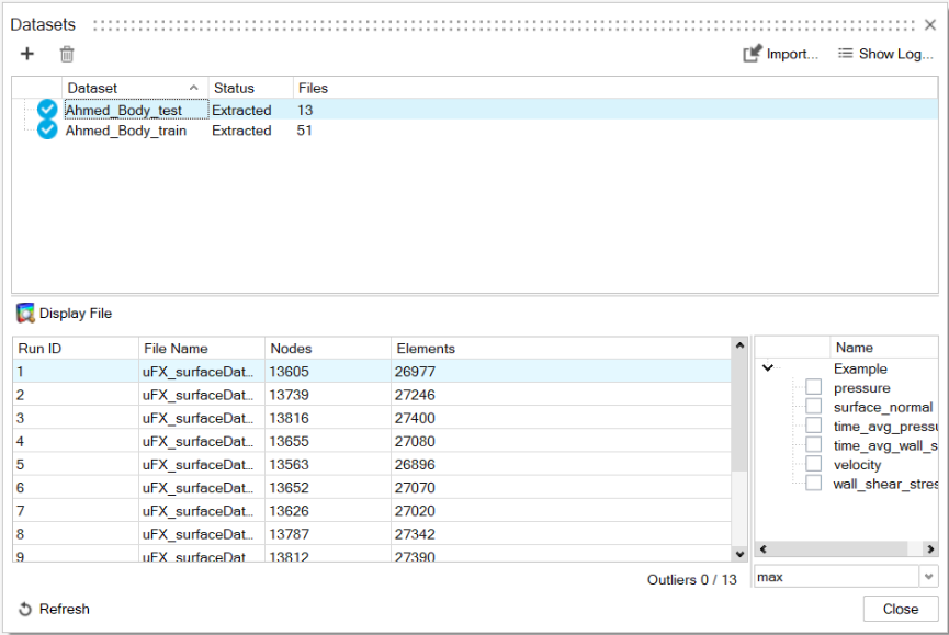 Note: Notice that due to the use of the Enable Train Test Split option, two datasets are created, one for training and one for testing.
 The Train Model dialog opens.
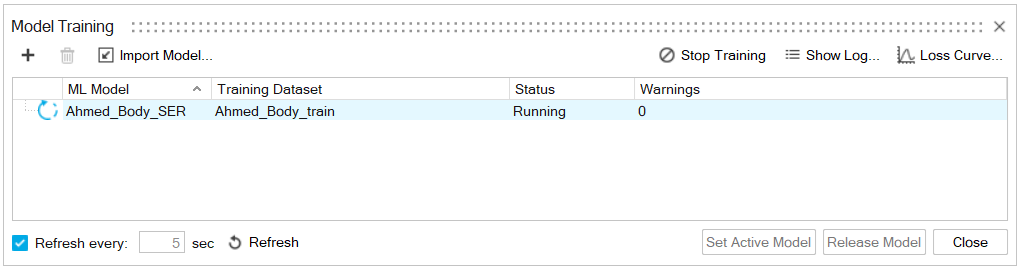 The Model Training dialog opens.
 to expand the drop-down menu. For Buffer
% set a value of 30.
to expand the drop-down menu. For Buffer
% set a value of 30.


 The Train Model dialog opens.
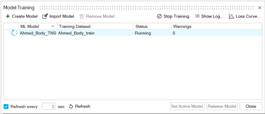 Note: Once the Status changes to Running, click on Show Log to inspect the training log file or click on Loss Curve to monitor the progression of the training and validation losses.
 The Test Model dialog opens.