Use HyperStudy for Data Curation and Pre-Processing
Tutorial Level: Beginner In this tutorial, you will use HyperStudy for data visualization, outlier detection, and .json file generation.
Restriction: This tutorial takes place entirely in HyperStudy. You must have HyperStudy installed to complete this tutorial.
HyperStudy can be used for visualizing and analyzing the
available training data. This is done by iterating through the existing
files.
Note: Since it was added in 2025, the PhysicsAI ribbon in HyperStudy creates a seamless
integration from data generation, process automation, curation to
prediction.
Before you begin, copy the file(s) used in this tutorial to your
working directory.
Perform the Study Setup
In this step, you create a study, add a model, and import .h3d files.
- Launch HyperStudy.
-
Start a new study in the following ways:
- From the menu bar, click .
- On the ribbon, click
 .
.
-
Add a model.
Figure 1. 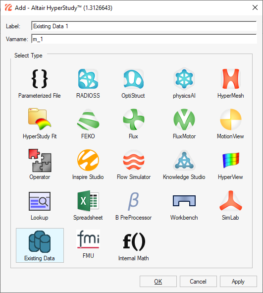
- In the Solver Input File field, enter arm.h3d.
-
Import .h3d files.
-
Click Add All Files.
The available .h3d files are moved to the Chosen Files area.
Figure 2. 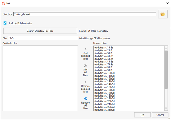
-
Click Add All Files.
Perform Nominal Run
- From the Model Tree, click to open the Test Models task.
- Click Run Definition.
Create 3D Visualization
- From the Model Tree, click to open the Define Output Responses task.
- From the Media Sources tab, click Add Media Source.
-
In the File field, click
 and browse
and select the arm.h3d file in
setup-run001\m_1.
and browse
and select the arm.h3d file in
setup-run001\m_1.
-
In the Tool Settings field, click
 .
The Media Source Builder dialog opens.
.
The Media Source Builder dialog opens. -
For Type, select Displacement and click
OK.
Figure 3. 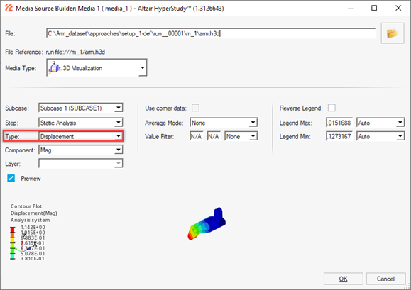
-
Add a second media source by repeating steps 2 - 5, but select Element Stresses (2D & 3D) as the
Type.
Figure 4. 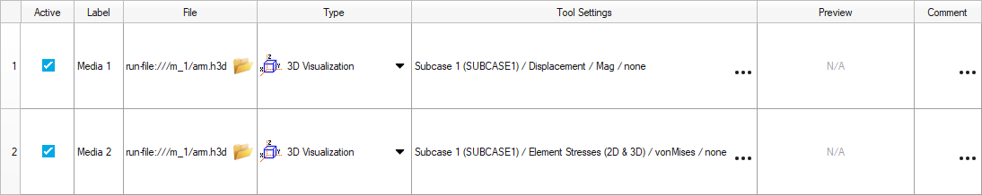
Create KPIs
In this step, you will create KPIs to analyze the results numerically.
- From the Data Sources tab, click Add Data Source.
-
In the File field, click .
The Data Source Builder dialog opens.
-
In the File field, click and browse
and select the arm.h3d file in
setup-run001\m_1.
- For Tool, select Read Simulation.
- For Type, select Displacement (Grids).
-
For Components, select MAG.
Note: This reads all the displacement values for all the nodes into a single vector from which values can be queried.
-
Click OK.
Figure 5. 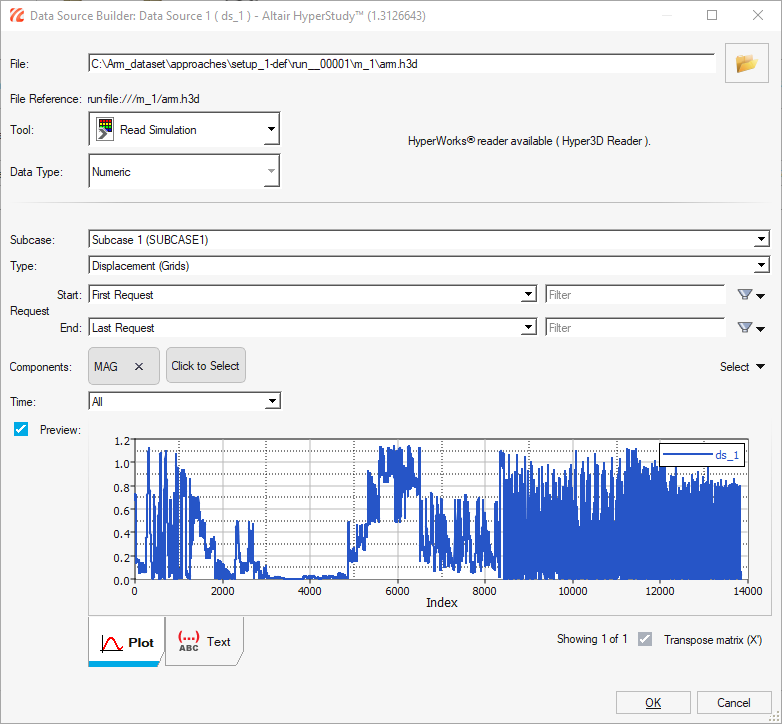
-
Create two more data sources using the information in Table 1 by repeating steps 1 - 7.
Table 1. Data Source Details File Tool Type Components arm.h3d Read Simulation Element Stresses (3D) vonMises (2D & 3D) arm.h3d Read Simulation Element Strains (3D) vonMises (2D & 3D) Figure 6. 
- Click Evaluate.
Create and Evaluate Output Responses
- From the Define Output Responses tab, click Add Output Response.
- In the Label field, enter max_disp.
-
In the Expression field, click .
The Expression Builder dialog opens.
-
In the Expression field, enter max(ds_1).
Note: Verify that ds_1 corresponds to the data source for displacement.
Figure 7. 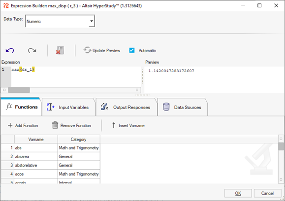
- Click OK.
-
Create five more output responses using the information in Table 2 by repeating steps 1 - 5.
Table 2. Output Response Details Label Expression min_disp min(ds_1) max_stress max(ds_2) min_stress min(ds_2) max_strain max(ds_3) min_strain min(ds_3) -
Click Evaluate.
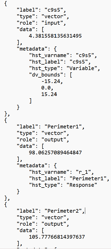
These are the six KPIs on which the training points can be evaluated.
Figure 8. 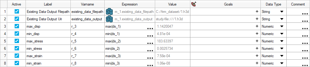
Create and Run DOE
-
Add a DOE.
Note: A DOE must be created from the setup to iterate through all the files identified in step 5 of Perform the Study Setup. The DOE will create as many DOE runs as the number of files in the list.
- In the Study Explorer, right-click and select Add from the context menu.
- In the Add dialog, select DOE.
- For Definition from, select Setup and click OK.
- Go to the step.
- In the Settings tab of the Specifications step, verify the Number of Runs matches the number of files identified in the Setup.
- Click Apply.
- Go to the step.
- Click Evaluate Tasks.
- Go to the step.
-
In the Media tab, review the evaluation results.
All the training files can be simultaneously loaded. You can inspect the plots visually using the media sources created earlier. As seen in , run IDs 31 and 32 have erroneous displacement and stress values. Hence, they are clear outliers.
Figure 9. 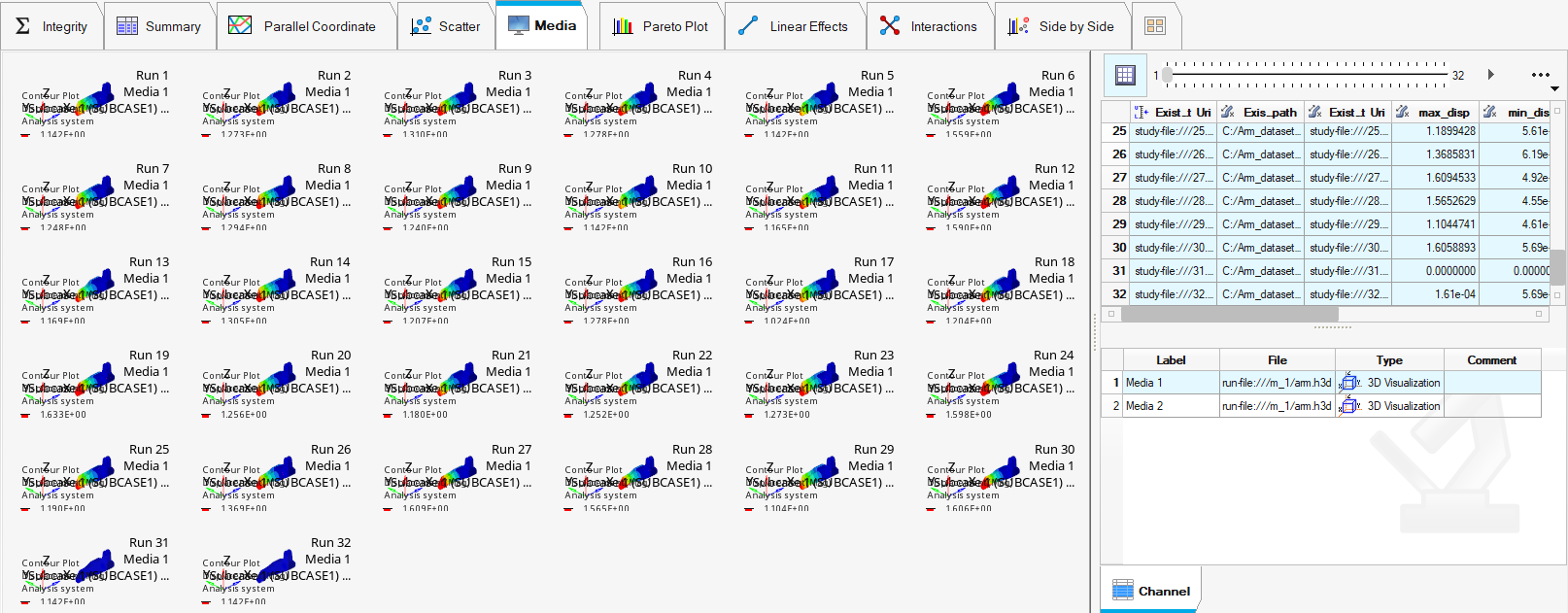
-
In the Parallel Coordinate tab, inspect the training data using the KPIs and
select the metrics created in step 6 of Create and Evaluate Output Responses.
Again, runIDs 31 and 32 are clear outliers.
Figure 10. 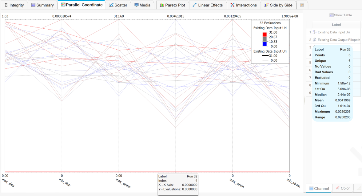
Generate Json Files
In this step, you will generate the .json files required for custom global inputs and outputs by using the genrpt_hst_paishape.py extension in the installation directory of HyperMesh.
-
If necessary, load the genrpt_hst_paishape.py
extension.
-
In the new row, click and browse and select the genrpt_hst_paishape.py
extension from
\hwdesktop\hw\eds\etc\hst_reports.
Figure 11. 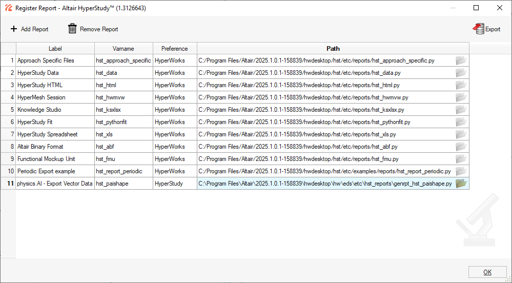
-
In the new row, click
- Go to the step.
- Select physics.AI - Export Vector Data and click Create Report.