Learn more about the best practices for training and using PhysicsAI models.
Problem Definition
The problem definition is the scope of the problem to be solved.
It is impossible to have a single PhysicsAI model that
can do everything. As such, it is important to define the scope by answering the
following questions before getting started:
What does the model need to predict?
Identify the handful of fields or KPIs that the model should predict
with sufficient accuracy.
What is the expected accuracy?
This is the gage for determining the success/failure of the model. The
error metric (such as mean average error (MAE) or other) and its
threshold magnitude (like 5%, 10%, and so on) from the true (simulation
result) is required.
How much data is available?
It is impossible to know how much data would be required at the onset.
It is advisable to collect as many relevant data points as possible. If
too few data points are available, generation of synthetic data should
be considered. If more data is difficult to come by, high accuracy
expectation may not be practical.
Data Preparation
A PhysicsAI model is only as good as the data used to
train it.
The recommended practices to create good datasets can be summarized as follows:
Ensure that the training dataset is sufficiently large and varied.
For small training datasets, consider skipping validation dataset creation.
Small training sets mean very small validation sets, which risk
overfitting.
Curate data by removing outliers.
Downsize training files by selecting results for reduced memory consumption and
processing time.
Synthetically generate data to augment existing data if needed.
Ensure data is rotationally and translationally aligned.
Ideally, a training dataset should contain a sufficient number of data points and
should be varied enough to be a good representative of the design space.
Some good practices for data preparation include: curation, down selecting, and
partitioning.
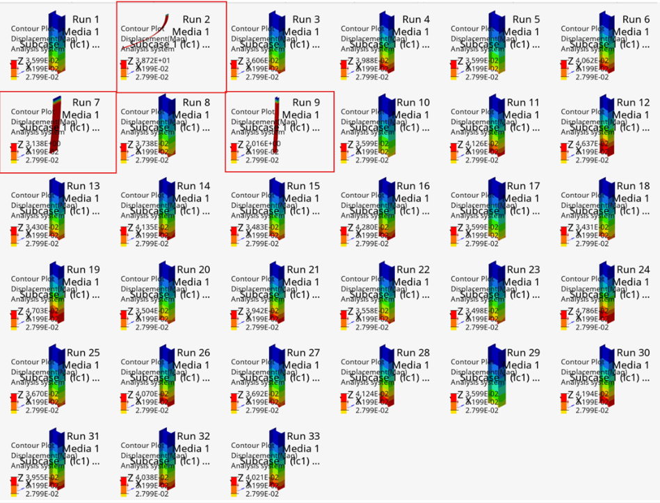
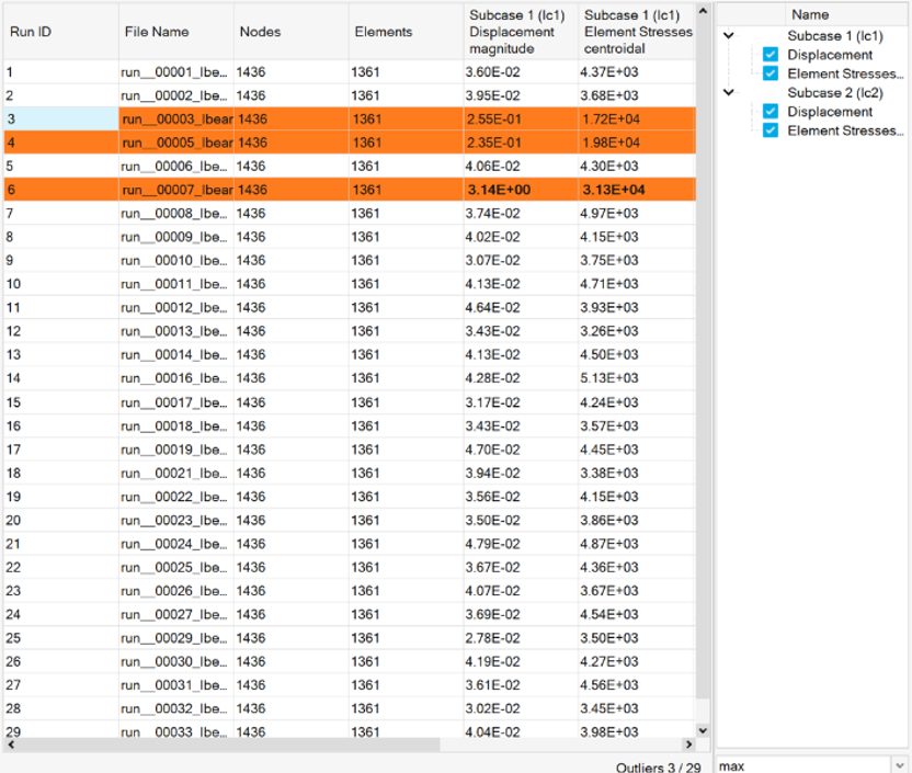
Curation
Inclusion of outliers can introduce noise and depreciate the prediction accuracy.
Hence, the available training data needs to be carefully curated by excluding the
outliers. This is a manual process but tools available within HyperMesh (dataset outlier detection) and HyperStudy (parallel plots, 3D visualization, KPI tracking)
can be used. Outliers can be identified using multiple criteria. These include but
are not limited to:
Inconsistent number or type of parts
Inconsistent and/or unequal number of timesteps
Rotational and/or translational variance (before version 2025.0) in the
orientation of parts
Additionally, incompatibility can also render some data invalid. These include but
are not limited to:
Unsupported element types or results
Subcase and result inconsistency
Down Selecting
Dataset creation by parsing available simulation results is a time intensive process.
Typically, native result files have large memory footprints with multiple load cases
and parts included. The time required to process these can be long. As such, only
the results of interests, such as for selected parts and timesteps, can be extracted
by translating into .h3d files
using HVTrans. These translated files are much quicker to process due to their
smaller size.
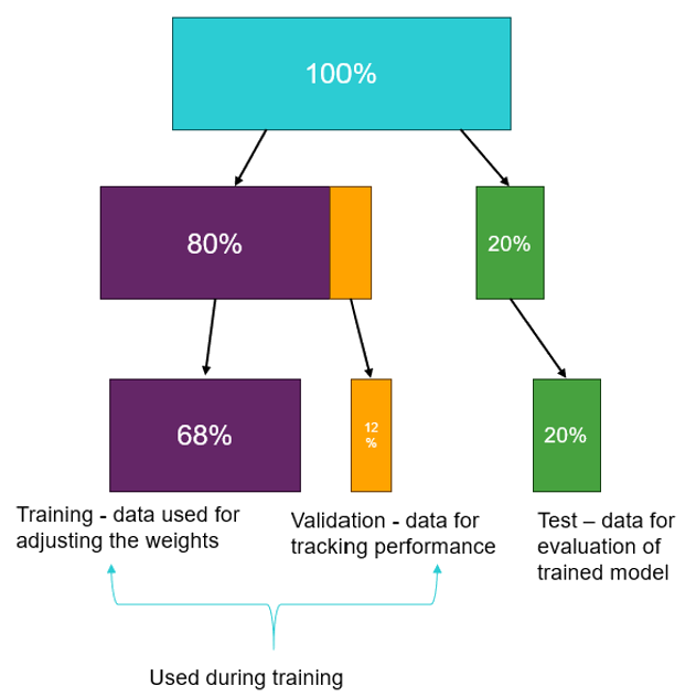
Partitioning
Typically, the filtered-out training data is partitioned into train, validation, and
test datasets. PhysicsAI automatically does this
partitioning using the following rules:
The entire dataset is split into train and test sets based on the fraction input
(default is 0.80- 80% for training and 20% for testing).
The train set from the previous step is further split into train and validate
sets (fixed value of 0.85 – 85% for training and 15% for validation). A
validation set is only created if the training set is more than 13, otherwise
only the training dataset is used.
Figure 3. Partitioning of Available Data
The role of a validation dataset is to avoid overfitting; the network is adjusted for
the training data but the loss is tracked for the validation dataset. This ensures
that the model can predict well for most data points in the design space and not
just the training data points. If the original dataset is small, the validation
dataset can be too small (<5) which can result in it being an incomplete
representation of the design space. As such, more data is needed for certain
problems to get a sufficiently large validation dataset for a better performing
model.
Identify Inputs and Outputs
Determining the correct inputs and outputs is key to a well-trained PhysicsAI model.
Input Selection
Including inputs which are not changing between the data samples adds
redundant variables.
On the other hand, not including the inputs which are changing would
confuse the model as it will observe different results for the same or
reduced set of variables.
For example, if the geometry is constant, but the loads are
changing, then it is imperative to include the loads (using
either the global or nodal hooks) as a variable. Otherwise, the
model will learn to predict the same output for all the data
points.
Some scenarios qualify for both global and nodal inputs. For those, the
global option is preferred as the input is more emphasized than the
nodal option.
Part labels can be used to distinguish between different parts in a
training data point. For example, rigid support vs deforming part or
parts made of different materials, and so on.
For the auxiliary files
(.json/.csv) maintain the
naming convention, data structure, label consistency, and required
fields per the requirements of the python hooks.
Output Selection
Multiple outputs can be selected for training. However, selecting too
many outputs would result in poor overall accuracy due to tradeoffs
between competing results. The recommended upper limit on the number of
outputs that the model should be trained on simultaneously is three,
although the GUI does not stop you from going beyond that.
You can choose between a single contour, multiple contours, a single
vector, or a single vector and multiple contours.
Multiple vector selection is currently not supported. For derived curve
responses such as force vs displacement, additional post-processing in
other tools such as HyperGraph, HyperStudy, or Compose is necessary.
For custom output curves with a large number of points and variation, it
is best to either down sample the data or use a moving average.
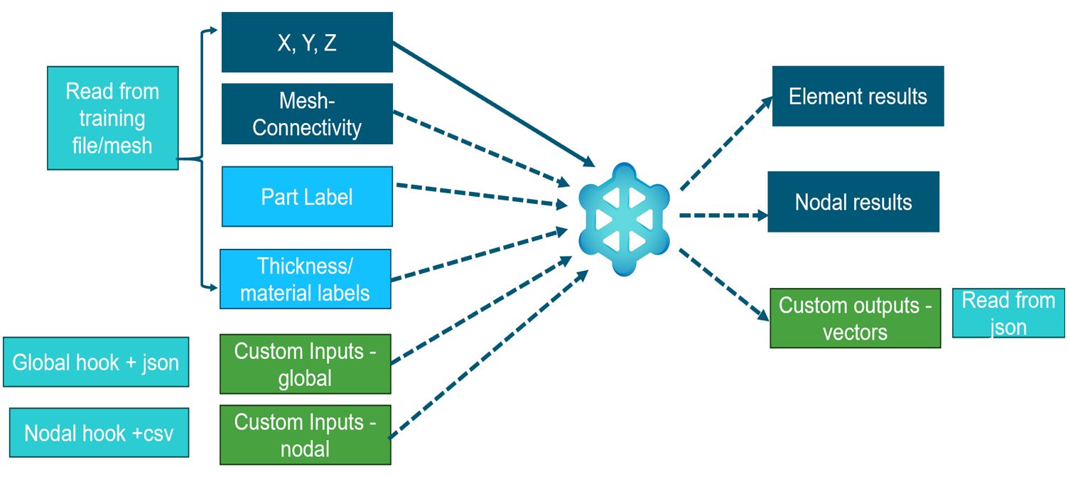
PhysicsAI supports the following inputs and outputs
for training the models.
Figure 4. Inputs and Outputs to a PhysicsAI Model
Inputs
Nodal coordinated (default and always selected)
Part labels (default but unselected): to distinguish between
rigids/non-rigids or different materials.
Thickness and material labels (using Extract Simulation Properties): enabled
if supported solver decks are present. For a list of supported solver decks,
refer to Frequently Asked Questions.
Global inputs (custom input - optional): input using a
.json file and read using a python hook. These are
applied to each node and hence are global. Typically used to input a global
property such as material characteristics, global boundary conditions, and
so on.
Nodal inputs (custom input - optional): input using a
.csv file and read using a python hook. These are
applied to specific nodes. Typically used to input node varying properties
such as nodal loads and other boundary conditions.
Outputs
Contour/field results (optional): identified by load case and result label.
Directly imported from the training simulation files.
Vector results (custom output – optional): used for curves or KPIs and
identified using a text label. Input using .json files.
The vectors are plotted against indices. Hence, the onus is on you to ensure
that the vector lengths and timesteps are consistent.
Generation of the auxiliary files for custom inputs and outputs
(.json and .csv files) is typically
done outside PhysicsAI using scripting or other tools
such as HyperStudy or Compose. The onus is on you to generate these files.
Training
Learn more about the recommended guidelines during PhysicsAI model training.
The recommended guidelines during PhysicsAI are:
Train with a single data point to get started using the default
hyperparameters. If the model is unable to predict for the single point it
trained on, then it may not learn to predict on the entire training set
either.
Hyperparameter tuning cannot fix bad data. Modify hyperparameters only after
issues with data have been eliminated. Ensure that the required memory does
not exceed the available while increasing the values.
Table 1. Typical Ranges
Hyperparameter
GCNS
TNS
Width
10-300
48-256
Depth
1-10
4-10
Epochs
100-5000
Learning Rate
1E-3-1E-6
Sections
X
16-128
Attention heads
X
4-16
Track the loss curve to capture the trend, not to estimate accuracy. The
effectiveness of the fit or model accuracy should always be evaluated by
testing and not from the loss curve as the latter is difficult to interpret.
The MAE (or other human interpretable metric) produced during testing is
more intuitive and is a holistic evaluation including the conformance of
distribution, presence of hotspots and so on can be made.
Since the required number of epochs is hard to predict, a large number of
epochs can be specified, and early stopping can be used for terminating the
training on convergence. Typically, transient results and KPIs/curve
predictions require more epochs (>5000).
Transfer learning should only be used to tune an existing model to a new but
similar dataset for optimal results. The new model will be accurate only for
the new dataset and not the original due to catastrophic forgetting during
the second training.
PhysicsAI has the following options for training:
Architecture
Hyperparameters
Diagnostics: logs and loss curves
Transfer learning
Architecture
PhysicsAI offers three separate training
architectures:
The graph-based Graph Context Neural Simulator (GCNS)
The default option and the only option available in 2024.1 or
earlier
On CPUs, GCNS typically runs faster than TNS
Requires less memory than GCNS
More stable during training
The transformer-based Transformer Neural Simulator (TNS)
Only available in version 2025.0 or later
Typically, runs faster than GCNS on GPUs
Has a larger number of parameters than GCNS
Is mesh-size invariant and is particularly advantageous for CAD based
predictions
Results in smoother contours
Recommended for transient, large deformation simulation
The Shape Encoding Regressor (SER)
Only available in versions 2025.1 or later
Only works for vector outputs (KPI/curves, not fields)
Much faster than the other two architectures
In Table 2, the symbols have the following meaning:
✓: the architecture has the capacity.
+ and -: indicate relative performance on the given criteria.
Table 2. Architecture Comparison
GCNS
TNS
SER
Contour Output
✓
✓
KPI or Curve Output
✓
✓
✓
Mesh Input
✓
✓
✓
CAD Input
✓
✓
Custom Inputs
✓
✓
Contour Smoothness
✓
NA
Training Time
-
+
Training Stability
-
+
GPU Memory
+
-
NA
Hyperparameters
These are the settings used for controlling the training and determine the duration
and the memory requirements. Hyperparameter tuning cannot compensate for bad
data.
The details for these are as follows:
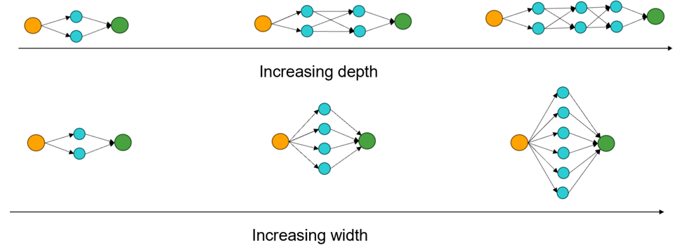
Width: controls the width (number of neurons in starting layer). Higher
widths result in better resolution (capturing the finer details in the
model) but also increases the memory requirements. The typical range of
width values is 10-300 for GCNS and 48-256 for TNS.
Depth: controls how deep the neural network is (number of layers). Higher
depth results in increased complexity of the model (analogous to order of
polynomial). Typical range of width values is 1-10 for GCNS and 4-10 for
TNS.Figure 5. Effect of Increasing Width and Depth on the Underlying Neural
Network Architecture
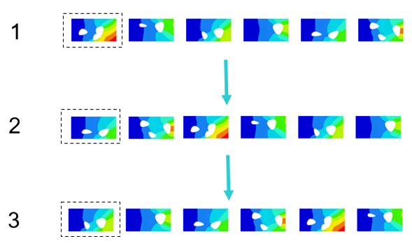
Epochs: an epoch involves training on each data point once. Thus, the number
of epochs specifies the number of training iterations. Complex problems need
longer epochs. If you are unsure about how many epochs are needed, a large
value (>5000 epochs) could be selected with early stopping enabled. Figure 6. Sequential Training During Epochs Early stopping checks if there is no improvement after the specified
number of epochs (patience) before terminating the training. PhysicsAI uses the best epoch (lowest validation loss
or, if not available, the training loss) and not the last epoch as the final
configuration of the model.
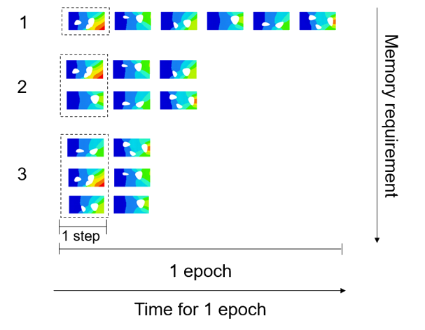
Batch size: determines how many data points are seen at once. Larger batch
sizes lead to faster training but might negatively affect accuracy. The
batch size should be tuned for each problem. The batch size defaults to
1.Figure 7. Effect of Batch Size on Memory Requirements and Time Per
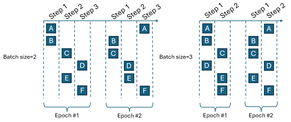
Epoch Within an epoch, batches of data are passed to the learning model in a
series of steps. Each single piece of data will be in only one step during
each epoch. In each epoch, the data is randomly shuffled into steps. Figure 8
illustrates a training with six data points (A-F) to compare the effect of
batch size. When the batch size is two, each epoch contains three steps and
requires six overall steps in the two epochs. In contrast, when the batch
size is three, each epoch contains two steps and requires four overall steps
in the two epochs. Using a batch size of three requires less overall steps,
but at the expense of larger memory requirement to load the batch into
memory. The optimal batch size depends on the problem being solved and can
truly be determined through trial and error.Figure 8. Progression of Training Inside Each Epoch
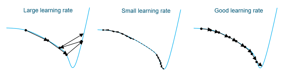
Learning rate: determines the step size by which the parameters are adjusted
during each step of every epoch. Adaptive learning rates are more robust
than constant ones. Adaptive learning rate follows the cosine decay law
where you specify the final fraction that the learning rate reduces to.
Typically, the last parameter that should be modified as the default value
should be sufficient for most problems.Figure 9. Effect of Varying Learning Rates The optimum learning rate is large enough to quickly move closer to
the optimum but small enough to not skip the optimum value.
Sections: a TNS parameter controlling the contextual resolution of the
neural network. It is typically set between 16-128.
Heads: a TNS parameter controlling the multi-headed attention. It is
typically set between 4-16. The higher the number of heads, the better the
expressivity.
Diagnostics: Logs and Loss Curves
PhysicsAI outputs both a text log and a graphical
representation of the loss values during training. Note that the loss is measured as
the Mean Square Error (MSE) in transformed units. It is difficult to know what a
good MSE value is or how well the model has trained by purely looking at the loss
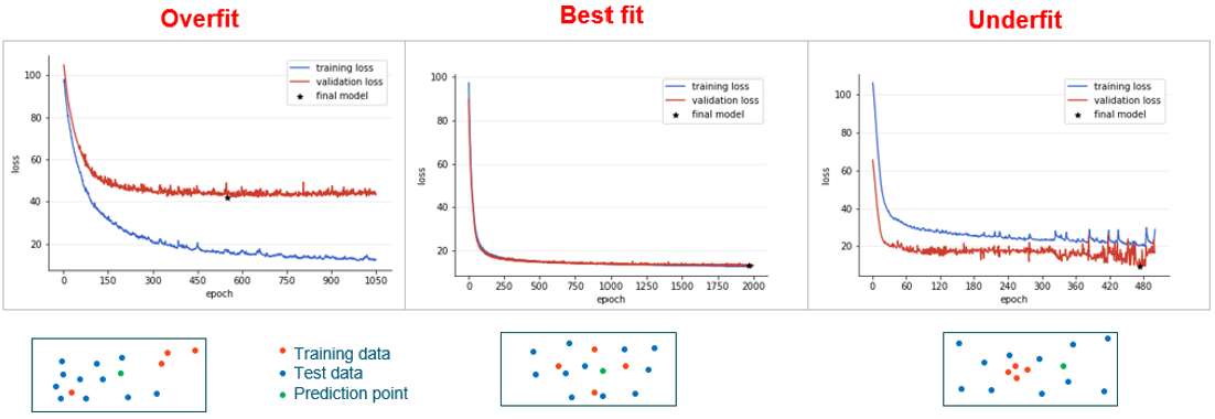
curve. However, overfitting, underfitting, or noisy models can be identified.
Figure 10. Different Types of Loss Curves
If the validation loss is much higher than the training loss, then the model is
overfit to the training data. This implies that the model is not generic enough
for the design space. This could possibly be due to a small or skewed
dataset.
An optimally trained model will have both the training and validation losses
converge closer to each other.
If the validation loss is lower than the training loss, then the model is
possibly underfit or the validation set is not diverse enough to represent the
design space.
Transfer Learning
Transfer learning means learning from a previous trained model. It essentially uses
the reference model as the starting point for the training instead of a random
configuration. This is useful for adapting a model to the current dataset. Thus, it
is important to ensure that the available model is relevant for the current dataset.
Additionally, the inputs need to be consistent.
Figure 11. Example of Transfer Learning Where a Generic Model is Adapted for a New
Dataset
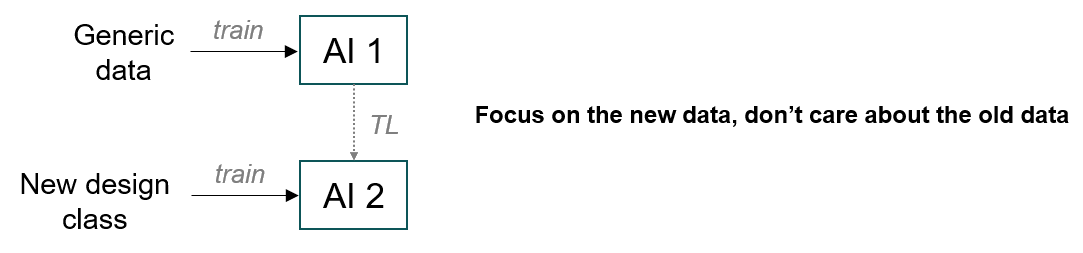
Transfer learning should be used to:
Repurpose a PhysicsAI Model
Adapt a generic model for a new class of designs.Figure 12. Valid Uses of Transfer Learning
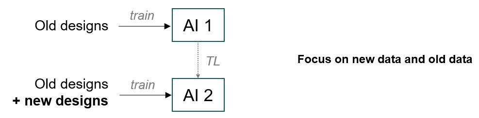
Update an Existing PhysicsAI Model
Use the old model and new data to create an improved model.Figure 13. Valid Uses of Transfer Learning Continued
Evaluation
Learn more about the recommended guidelines during PhysicsAI evaluations.
Some good practices for testing and predicting are:
Testing is the recommended way to evaluate the accuracy of the model on a
specified test dataset.
The test dataset should be a good representation of the design space.
Should be unseen but relevant data
Should have true results available
The accuracy or goodness of a fit should not be restricted to a singular
numerical value such as MAE, but rather be holistic considering the distribution
of the result values, smoothness of results, and so on.
One or more error metrics can also be considered.
Prediction should be made on CAD or meshes which are similar (in terms of the
number and type of parts, material IDs, and geometric and non-geometric
inputs).
If hooks are used during prediction, make sure that the
.json or .csv file is named and
located per the requirements of the hooks.
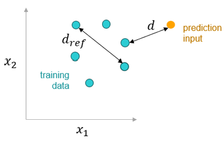
The similarity score is a projection of confidence into the accuracy of the prediction.
A similarity score of 1 indicates that the new design geometrically
matches at least one of the samples in the training dataset.
The worst value is –inf and indicates a completely different
geometry.
The prediction is saved in an .h3d file with no mesh information (for contours) and
.json/.XY files (for KPIs and
curves).
Evaluation using a PhysicsAI model can be done in two ways:
Test
This is done with the objective of evaluating a PhysicsAI model. This is done using the Model
Testing tools and a test dataset wherein the true results are known, and
the predicted results can be compared based on key error metrics such as
MAE. Additional metrics are available inside the testing log file.
Predict
This is used for evaluating new designs and the true results are not
available to make comparisons. A similarity score is displayed to
indicate the confidence in the accuracy of the results based on the
geometrical similarity of the new design with the datapoints in the
training dataset.
Figure 14. Similarity Score Calculation
Similarity score:
1.0
Equivalent to training sample
0.0
As far from the nearest training point as any two training points are
from each other