Train models using any physics, any mesh, and without design variable
parametrization.
Note: Training times vary significantly depending on various factors, such as:
Inclusion of a Dataset (number of samples and number of elements and
time steps per sample)
Model specifications (model size, hyperparameters, number of training
epochs)
Hardware (processor speed, RAM, access to GPU)
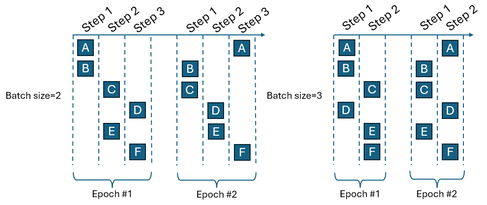
Training is an iterative process. One complete iteration is known as an epoch. Within
an epoch, batches of data are passed to the learning model in a series of steps.
Each single piece of data will be in one (and only one) step during each epoch. In
each epoch, the data is randomly shuffled into steps. Figure 1 illustrates a training
with six data points (A-F) to compare the effect of batch size. When batch size is
two, each epoch contains three steps and requires six overall steps in the two
epochs. In contrast when the batch size is three, each epoch contains two steps and
requires four steps in the two epochs. Using batch size of three requires less
overall steps, but at the expense of larger memory requirement to load the batch
into memory. The optimal batch size depends on the problem being solved and can
truly be determined through trial and error.Figure 1.
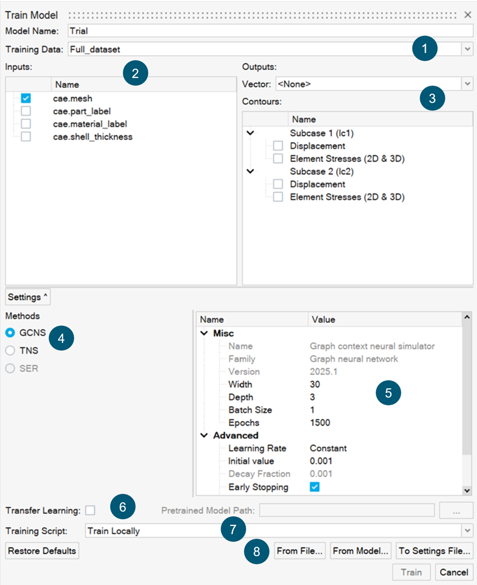
From the PhysicsAI ribbon, select the Train
an ML Model tool.
Figure 2.
The Train Model dialog opens. See Navigate the Train Model GUI for
more information about the Train Model dialog.
Define the training details and click Train.
Enter a model name.
For Training Data, select the created or existing Train Dataset.
Select Inputs and Outputs.
Multiple responses can be selected for training.
Select a Training Script.
Note: Options to train using Altair One
compute resources will appear when two requirements are met:
The project is saved to Altair One Drive.
At least one visible compute appliance in Altair One has an installed version
of PhysicsAI that is consistent
with the edge client version of PhysicsAI.
Specify the hyperparameters of the training process, such as the number
of epochs or learning rate.
Tip: If desired, transfer learning can also be
enabled.
Transfer learning involves using the knowledge from
an existing PhysicsAI model while
training a new model. It can be beneficial in cases where too
few data points are available for training a new model from
scratch. To enable transfer learning, the new PhysicsAI model should have the exact
same width, depth, and input features.
Note: You can
hover over the hyperparameter names to read their
description.
Hyperparameters will affect the quality of a
trained model. The optimal set of hyperparameters will vary from
problem to problem. Running experiments to the tune the
hyperparameters to maximize model performance is an important
last step in a complete PhysicsAI
process.
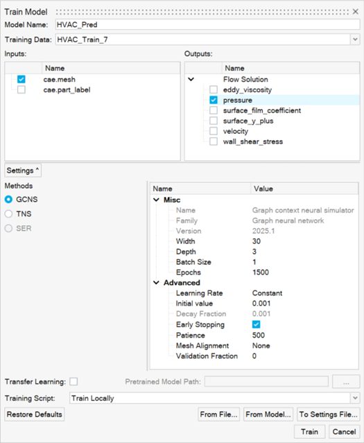
Figure 3. PhysicsAI has three AI methods
available for training: Graphical Context Neural Simulator (GCNS), which
is the default option, Transformer Neural Simulator (TNS), and Shape
Encoding Regressor (SER). For more details, refer to Frequently Asked Questions.
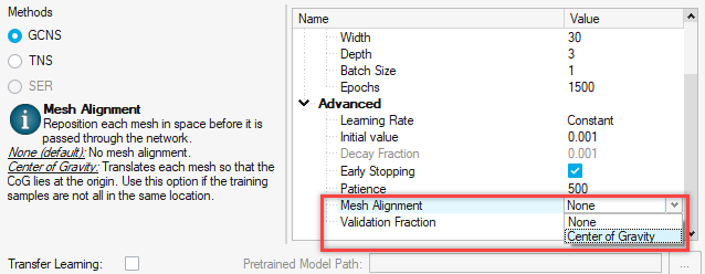
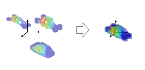
Tip: For
meshes which are translated in space, these can be realigned using
the Mesh Alignment option during model training.Figure 4. Figure 5.
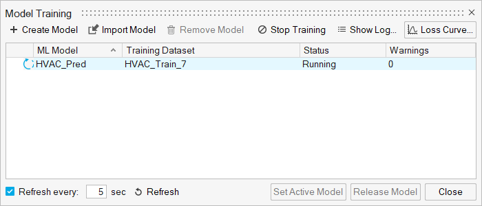
The Model Training dialog
opens.
Review the status in the Status column.
Tip: Once the status changes to Running, you can view the training
logs by clicking Show Log.
Figure 6.
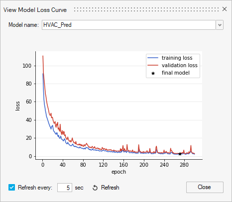
Optional: Click Loss Curve to view the training of a validation
loss curve.
The curves are useful to visualize the progress of the training process. In a
well fit model, the training and validation losses become nearly identical. If
validation never approaches the training loss, this is indicative of
underfitting; increased training time can leave files d to improved model
performance. A validation loss that approaches the training loss but diverges
higher likely indicates overfitting; the point of low validation loss is the
ideal model to avoid loss of generalization. For more information, see Best Practices for PhysicsAI.
Note: The validation curve only appears if there are at least 15
samples.
Figure 7.
Train Remotely on an HPC
Train a PhysicsAI model on a remotely on a different machine than the one running the
PhysicsAI GUI.
To train models remotely, you
will need:
Access to a remote machine with the Engineering Data Science (EDS) application
installed
PuTTY installed on your local machine
A training script (details below)
A mapped drive which can be accessed by both your local machine and the HPC.
This is required so that your locally created datasets are visible to the HPC
during training.
A common reason for remote training is to harness an HPC with a GPU, which can
accelerate training significantly.
Install the EDS application from the Altair One
Marketplace to your HPC.
Create an SSH connection.
Launch PuTTY on your local machine and connect to the HPC via
SSH.
Save the connection, for example:
my_PhysicsAI_hpc.
Important: If you are required to enter a password while logging in
via PuTTY, you will need to setup RSA keys before continuing. Once you can
login via PuTTY without entering a password, you may continue.
Write a training script for your HPC using the following template.
This example uses the qsub command from PBS on Windows. For Windows, the script should have the
.bat extension. If your local machine is running Linux,
you will need to write a script with equivalent functionality on Linux with a
.sh extension.
@echo off

SETLOCAL

REM ------------------------------------------------------------------------------
REM Copyright (c) 2021 - 2021 Altair Engineering Inc.  All Rights Reserved
REM Contains trade secrets of Altair Engineering, Inc.  Copyright notice
REM does not imply publication.  Decompilation or disassembly of this
REM software is strictly prohibited.
REM ------------------------------------------------------------------------------


REM ------------------------------------------------------------------------------
REM USER SETTINGS
REM ------------------------------------------------------------------------------

REM HPC Setup
set sess=<<HOST NAME>>
set user=<<USER NAME>>

REM PBS Requests
set pbs_requests=-q a100 -N PhysicsAI_shape  -j oe -l select=1:ncpus=8:mem=257940mb:ngpus=1

REM Windows -> Unix Mapping
set win_map=\\<<SERVER IP>>\data\ds
set unix_map=/data/ds

REM PhysicsAI Installation Settings
set install_loc=<<HW INSTALL LOCATION>>hwdesktop/hw/eds/bin/linux64/edspy.sh

REM PBS Install Location
set sub_cmd=/altair/pbsworks/pbs/exec/bin/qsub


REM ------------------------------------------------------------------------------
REM SCRIPT START
REM ------------------------------------------------------------------------------
REM Get whole input line
set line=%*


REM Map windows paths to unix
set unixmap=%win_map%=%unix_map%
set unixmap=%unixmap:\=/%
set submit_line=%line:\=/%
setlocal EnableExtensions EnableDelayedExpansion
set submit_line=!submit_line:%unixmap%!
echo %line%


echo ---UNIXMAP---
IF ["%unixmap%"] == [""] GOTO :RUN
setlocal EnableExtensions EnableDelayedExpansion

:RUN
echo ---PLINK SETTINGS---
echo user = %user%
echo sess = %sess%


echo ---PAI-SHAPE SETTINGS--
echo install_loc = %install_loc%
echo submit_line = %submit_line%


REM -----------------
REM Run QSUB
REM -----------------
set qsub_command_string='%install_loc% %submit_line%'

REM Write File for submission
echo plink -batch -load %sess% -l %user% -batch "echo %qsub_command_string% > pai_qsub.txt"
plink -batch  -load %sess% -l %user% -batch "echo %qsub_command_string% > pai_qsub.txt"

REM Submit file
plink -batch  -load %sess% -l %user% -batch "%sub_cmd% %pbs_requests% pai_qsub.txt"
echo plink -batch -load %sess% -l %user% -batch "qsub %pbs_requests% pai_qsub.txt"

ENDLOCAL
Below is a Linux example.
This example script is setup under the assumption that you can already submit
from your command terminal.
#!/bin/tcsh

# ------------------------------------------------------------------------------
# USER SETTINGS
# ------------------------------------------------------------------------------

set pbs_requests="-q a100 -N PhysicsAI_shape  -j oe -l select=1:ncpus=8:mem=250000mb:ngpus=1"
echo ${pbs_requests}

# Hyperworks Install Location
set install_loc="/stage/hw/2024"
echo ${install_loc}


# PBS qsub install location
set sub_cmd="/opt/pbs/bin/qsub"


# ------------------------------------------------------------------------------
# SCRIPT START
# ------------------------------------------------------------------------------

set submit_line="$*"
echo submit_line = ${submit_line}

set edspy=\$'{'install_loc'}'"/altair/hwdesktop/hw/eds/bin/linux64/edspy.sh"

set qsub_command_string="export INSTALL_LOCATION=${install_loc};export install_loc=${install_loc}; ${edspy} ${submit_line}"
echo qsub_command_string = ${qsub_command_string};


# Write the qsub sumbmission script.
# If your home directory is not seen by the HPC, modify the location to be visible on the HPC or run command via ssh.
echo "${qsub_command_string}" > ~/pai_qsub.txt;

# Submit the qsub sumbmission script.
# If you cannot directly submit to pbs, run this command via ssh.
echo "qsub ${pbs_requests} pai_qsub.txt";
qsub ${pbs_requests} ~/pai_qsub.txt
Register the training script.
From the PhysicsAI ribbon, select the
Train an ML Model tool.
Figure 8.
The Train Model dialog opens.
For Training Script, select Register Training
Script.
The Add Training Script dialog
opens.
Click and browse and
select your training script.
Enter a name for your script and click OK.
Close the Train Model dialog.
Your preferences are saved and the
physicsai_solver_prefs.json file in your user directory
has been updated.
Install the NVIDIA CUDA toolkit and cuDNN library.
Once these tools are installed, the GPU will be used by default for both
training and predicting. You can verify this in the Task Manager by enabling the
cuda graph in the GPU Performance tab.
To use the CPU again, set CUDA_VISIBLE_DEVICES=-1 as an
environment variable.
Navigate the Train Model GUI
Figure 9.
Drop-down menu to select from available datasets.
Inputs selection based on available inputs from the dataset. Both native and
custom inputs are displayed here.
Input Feature
Description
cae.coord
Spatial coordinates used as a predictor of behavior.
It is recommended to always keep it on.
cae.part_label
Part name is used as a predictor of behavior. This is
valuable when working with large assemblies. In most
cases, it is recommended to keep it on. However, it may
make sense to turn it off in cases with inconsistent
part names.
cae.shell_thickness
The thickness of 2D shell elements is used as a
predictor of behavior. This is required when the dataset
has varying thicknesses between simulation models. This
feature is only available for supported solver decks
(for a list of supported solver decks, see Frequently Asked Questions) and requires the selection of
Extract Simulation Properties
during dataset creation. Solver input files must be in
the same directory as the associated output file and
have the same basename.
cae.material_label
Material name is used as a predictor of behavior.
This is required when the dataset has varied material
assignments between simulation models. This feature is
only available for supported solver decks (for a list of
supported solver decks, see Frequently Asked Questions)
and requires the selection of Extract
Simulation Properties during dataset
creation. Solver input files must be in the same
directory as the associated output file and have the
same basename.
Outputs selection based on the possible outputs contained within the
dataset. KPI and curve outputs are contained in a drop-down menu while field
outputs are shown in a tree chart.
When vector data is available, a vector
prediction option displays under Outputs. Vector data is provided
alongside the primary files selected during dataset creation. The vector
data should have the same basename as the primary data file, but with a
.json extension. An example of the
.json schema is shown below:
Architecture/method to be used for training. PhysicsAI has three architectures: Graph Context
Neural Simulator (GCNS), Transformer Neural Simulator (TNS), and Shape
Encoding Regressor (SER) (for KPI/curves predictions only, no field
predictions). For more information on these architectures, see Frequently Asked Questions or Best Practices for PhysicsAI.
Hyperparameters or training settings to be used. Five hyperparameters are
common to all architectures: width, depth, batch size, epochs, and learning
rate. Others are specific to each architecture. Click on the labels for a
description and recommended values. For additional information refer to the
Hyperparameters section and Best Practices for PhysicsAI.
Transfer Learning enables the use of a previously trained PhysicsAI model as a starting point, effectively
transferring the knowledge from the previously trained PhysicsAI model to the new PhysicsAI model which is being trained. To use
transfer learning, the inputs must be the same as the previously trained
model. For more information, see Best Practices for PhysicsAI.
Training Script is for specifying the execution location for the
training.
The specifications toolbar can be used to read the hyperparameter, inputs,
and output choices from an existing PhysicsAI
configuration file (.pscfg) or a PhysicsAI model file (.psmdl).
It can also be used to export the current settings as a configuration file
(.pscfg). This feature is useful to ensure that
settings can be kept consistent between different training rounds while
eliminating errors from manual operations.

 and browse and
select your training script.
and browse and
select your training script.